Tail-Recursive & Body-Recursive Function Performance Across Elixir & BEAM versions – what’s the impact of the JIT?

I’ve wanted to revisit “Tail Call Optimization in Elixir & Erlang – not as efficient and important as you probably think” (2016) for a while – so much so that I already revisited it once ~5 years ago to show off some benchee 1.0 features. As a reminder, in these the results were:

• body-recursive was fastest on input sizes of lists the size of 100k and 5M, but slower on the smallest input (10k list) and the biggest input (25M list). The difference either way was usually in the ~5% to 20% range.
• tail-recursive functions consumed significantly more memory
• we found that the order of the arguments for the tail-recusive function has a measurable impact on performance – namely doing the pattern match on the first argument of the recursive function was faster.

So, why should we revisit it again? Well, since then then JIT was introduced in OTP 24. And so, as our implementation changes, performance properties of functions may change over time. And, little spoiler, change they did.

To illustrate how performance changes across versions I wanted to show the performance across many different Elixir & OTP versions, I settled on the following ones:

• Elixir 1.6 @ OTP 21.3 – the oldest version I could get running without too much hassle
• Elixir 1.13 @ OTP 23.3 – the last OTP version before the JIT introduction
• Elixir 1.13 @ OTP 24.3 – the first major OTP version with the JIT (decided to use the newest minor though), using the same Elixir version as above so that the difference is up to OTP
• Elixir 1.16 @ OTP 26.2 – the most current Elixir & Erlang versions as of this writing

How do the performance characteristics change over time? Are we getting faster with time? Let’s find out! But first let’s discuss the benchmark.

The Benchmark

You can find the code in this repo. The implementations are still the same as last time. I dropped the “stdlib”/Enum.map part of the benchmark though as in the past it showed similar performance characteristics as the body-recursive implementation. It was also the only one not implemented “by hand”, more of a “gold-standard” to benchmark against. Hence it doesn’t hold too much value when discussing “which one of these simple hand-coded solutions is fastest?”.

It’s also worth nothing that this time the benchmarks are running on a new PC. Well, not new-new, it’s from 2020 but still a different one that the previous 2 benchmarks were run on.

System information

Operating System: Linux
CPU Information: AMD Ryzen 9 5900X 12-Core Processor
Number of Available Cores: 24
Available memory: 31.25 GB

As per usual, these benchmarks were run on an idle system with no other necessary applications running – not even a UI.

Without further ado the benchmarking script itself:

	map_fun = fn i -> i + 1 end
	inputs = [
	{"Small (10 Thousand)", Enum.to_list(1..10_000)},
	{"Middle (100 Thousand)", Enum.to_list(1..100_000)},
	{"Big (1 Million)", Enum.to_list(1..1_000_000)},
	{"Giant (10 Million)", Enum.to_list(1..10_000_000)},
	{"Titanic (50 Million)", Enum.to_list(1..50_000_000)}
	]
	tag = System.get_env("TAG")
	Benchee.run(
	%{
	"tail" => fn list -> MyMap.map_tco(list, map_fun) end,
	"body" => fn list -> MyMap.map_body(list, map_fun) end,
	"tail +order" => fn list -> MyMap.map_tco_arg_order(list, map_fun) end
	},
	warmup: 5,
	time: 40,
	# memory measurements are stable/all the same
	memory_time: 0.1,
	inputs: inputs,
	formatters: [
	{Benchee.Formatters.Console, extended_statistics: true}
	],
	save: [tag: tag, path: "benchmarks/saves/tco_#{tag}.benchee"]
	)

view raw bench_script.exs hosted with ❤ by GitHub

The script is fairly standard, except for long benchmarking times and a lot of inputs. The TAG environment variable has to do with the script that runs the benchmark across the different elixir & OTP versions. I might dig into that in a later blog post – but it’s just there to save them into different files and tag them with the respective version.

Also tail + order denotes the version that switched the order of the arguments around to pattern match on the first argument, as talked about before when recapping earlier results.

Results

As usual you can peruse the full benchmarking results in the HTML reports or the console output here:

Console Output of the benchmark

##### With input Small (10 Thousand) #####
Name                                  ips        average  deviation         median         99th %
tail +order (1.16.0-otp-26)       11.48 K       87.10 μs   ±368.22%       72.35 μs      131.61 μs
tail (1.16.0-otp-26)              10.56 K       94.70 μs   ±126.50%       79.80 μs      139.20 μs
tail +order (1.13.4-otp-24)       10.20 K       98.01 μs   ±236.80%       84.80 μs      141.84 μs
tail (1.13.4-otp-24)              10.17 K       98.37 μs    ±70.24%       85.55 μs      143.28 μs
body (1.16.0-otp-26)               8.61 K      116.19 μs    ±18.37%      118.16 μs      167.50 μs
body (1.13.4-otp-24)               7.60 K      131.50 μs    ±13.94%      129.71 μs      192.96 μs
tail +order (1.13.4-otp-23)        7.34 K      136.32 μs   ±232.24%      120.61 μs      202.73 μs
body (1.13.4-otp-23)               6.51 K      153.55 μs     ±9.75%      153.70 μs      165.62 μs
tail +order (1.6.6-otp-21)         6.36 K      157.14 μs   ±175.28%      142.99 μs      240.49 μs
tail (1.13.4-otp-23)               6.25 K      159.92 μs   ±116.12%      154.20 μs      253.37 μs
body (1.6.6-otp-21)                6.23 K      160.49 μs     ±9.88%      159.88 μs      170.30 μs
tail (1.6.6-otp-21)                5.83 K      171.54 μs    ±71.94%      158.44 μs      256.83 μs

Comparison: 
tail +order (1.16.0-otp-26)       11.48 K
tail (1.16.0-otp-26)              10.56 K - 1.09x slower +7.60 μs
tail +order (1.13.4-otp-24)       10.20 K - 1.13x slower +10.91 μs
tail (1.13.4-otp-24)              10.17 K - 1.13x slower +11.27 μs
body (1.16.0-otp-26)               8.61 K - 1.33x slower +29.09 μs
body (1.13.4-otp-24)               7.60 K - 1.51x slower +44.40 μs
tail +order (1.13.4-otp-23)        7.34 K - 1.57x slower +49.22 μs
body (1.13.4-otp-23)               6.51 K - 1.76x slower +66.44 μs
tail +order (1.6.6-otp-21)         6.36 K - 1.80x slower +70.04 μs
tail (1.13.4-otp-23)               6.25 K - 1.84x slower +72.82 μs
body (1.6.6-otp-21)                6.23 K - 1.84x slower +73.38 μs
tail (1.6.6-otp-21)                5.83 K - 1.97x slower +84.44 μs

Extended statistics: 

Name                                minimum        maximum    sample size                     mode
tail +order (1.16.0-otp-26)        68.68 μs   200466.90 μs       457.09 K                 71.78 μs
tail (1.16.0-otp-26)               75.70 μs    64483.82 μs       420.52 K       79.35 μs, 79.36 μs
tail +order (1.13.4-otp-24)        79.22 μs   123986.92 μs       405.92 K                 81.91 μs
tail (1.13.4-otp-24)               81.05 μs    41801.49 μs       404.37 K                 82.62 μs
body (1.16.0-otp-26)               83.71 μs     5156.24 μs       343.07 K                 86.39 μs
body (1.13.4-otp-24)              106.46 μs     5935.86 μs       302.92 K125.90 μs, 125.72 μs, 125
tail +order (1.13.4-otp-23)       106.66 μs   168040.73 μs       292.04 K                109.26 μs
body (1.13.4-otp-23)              139.84 μs     5164.72 μs       259.47 K                147.51 μs
tail +order (1.6.6-otp-21)        122.31 μs   101605.07 μs       253.46 K                138.40 μs
tail (1.13.4-otp-23)              115.74 μs    47040.19 μs       249.14 K                125.40 μs
body (1.6.6-otp-21)               109.67 μs     4938.61 μs       248.26 K                159.82 μs
tail (1.6.6-otp-21)               121.83 μs    40861.21 μs       232.24 K                157.72 μs

Memory usage statistics:

Name                           Memory usage
tail +order (1.16.0-otp-26)       223.98 KB
tail (1.16.0-otp-26)              223.98 KB - 1.00x memory usage +0 KB
tail +order (1.13.4-otp-24)       223.98 KB - 1.00x memory usage +0 KB
tail (1.13.4-otp-24)              223.98 KB - 1.00x memory usage +0 KB
body (1.16.0-otp-26)              156.25 KB - 0.70x memory usage -67.73438 KB
body (1.13.4-otp-24)              156.25 KB - 0.70x memory usage -67.73438 KB
tail +order (1.13.4-otp-23)       224.02 KB - 1.00x memory usage +0.0313 KB
body (1.13.4-otp-23)              156.25 KB - 0.70x memory usage -67.73438 KB
tail +order (1.6.6-otp-21)        224.03 KB - 1.00x memory usage +0.0469 KB
tail (1.13.4-otp-23)              224.02 KB - 1.00x memory usage +0.0313 KB
body (1.6.6-otp-21)               156.25 KB - 0.70x memory usage -67.73438 KB
tail (1.6.6-otp-21)               224.03 KB - 1.00x memory usage +0.0469 KB

**All measurements for memory usage were the same**

##### With input Middle (100 Thousand) #####
Name                                  ips        average  deviation         median         99th %
tail +order (1.16.0-otp-26)        823.46        1.21 ms    ±33.74%        1.17 ms        2.88 ms
tail (1.16.0-otp-26)               765.87        1.31 ms    ±32.35%        1.25 ms        2.99 ms
body (1.16.0-otp-26)               715.86        1.40 ms    ±10.19%        1.35 ms        1.57 ms
body (1.13.4-otp-24)               690.92        1.45 ms    ±10.57%        1.56 ms        1.64 ms
tail +order (1.13.4-otp-24)        636.45        1.57 ms    ±42.91%        1.33 ms        3.45 ms
tail (1.13.4-otp-24)               629.78        1.59 ms    ±42.61%        1.36 ms        3.45 ms
body (1.13.4-otp-23)               625.42        1.60 ms     ±9.95%        1.68 ms        1.79 ms
body (1.6.6-otp-21)                589.10        1.70 ms     ±9.69%        1.65 ms        1.92 ms
tail +order (1.6.6-otp-21)         534.56        1.87 ms    ±25.30%        2.22 ms        2.44 ms
tail (1.13.4-otp-23)               514.88        1.94 ms    ±23.90%        2.31 ms        2.47 ms
tail (1.6.6-otp-21)                514.64        1.94 ms    ±24.51%        2.21 ms        2.71 ms
tail +order (1.13.4-otp-23)        513.89        1.95 ms    ±23.73%        2.23 ms        2.47 ms

Comparison: 
tail +order (1.16.0-otp-26)        823.46
tail (1.16.0-otp-26)               765.87 - 1.08x slower +0.0913 ms
body (1.16.0-otp-26)               715.86 - 1.15x slower +0.183 ms
body (1.13.4-otp-24)               690.92 - 1.19x slower +0.23 ms
tail +order (1.13.4-otp-24)        636.45 - 1.29x slower +0.36 ms
tail (1.13.4-otp-24)               629.78 - 1.31x slower +0.37 ms
body (1.13.4-otp-23)               625.42 - 1.32x slower +0.38 ms
body (1.6.6-otp-21)                589.10 - 1.40x slower +0.48 ms
tail +order (1.6.6-otp-21)         534.56 - 1.54x slower +0.66 ms
tail (1.13.4-otp-23)               514.88 - 1.60x slower +0.73 ms
tail (1.6.6-otp-21)                514.64 - 1.60x slower +0.73 ms
tail +order (1.13.4-otp-23)        513.89 - 1.60x slower +0.73 ms

Extended statistics: 

Name                                minimum        maximum    sample size                     mode
tail +order (1.16.0-otp-26)         0.70 ms        5.88 ms        32.92 K                  0.71 ms
tail (1.16.0-otp-26)                0.77 ms        5.91 ms        30.62 K                  0.78 ms
body (1.16.0-otp-26)                0.90 ms        3.82 ms        28.62 K         1.51 ms, 1.28 ms
body (1.13.4-otp-24)                1.29 ms        3.77 ms        27.62 K         1.30 ms, 1.31 ms
tail +order (1.13.4-otp-24)         0.79 ms        6.21 ms        25.44 K1.32 ms, 1.32 ms, 1.32 ms
tail (1.13.4-otp-24)                0.80 ms        6.20 ms        25.18 K                  1.36 ms
body (1.13.4-otp-23)                1.44 ms        4.77 ms        25.00 K         1.45 ms, 1.45 ms
body (1.6.6-otp-21)                 1.39 ms        5.06 ms        23.55 K                  1.64 ms
tail +order (1.6.6-otp-21)          1.28 ms        4.67 ms        21.37 K                  1.42 ms
tail (1.13.4-otp-23)                1.43 ms        4.65 ms        20.59 K         1.44 ms, 1.44 ms
tail (1.6.6-otp-21)                 1.11 ms        4.33 ms        20.58 K                  1.40 ms
tail +order (1.13.4-otp-23)         1.26 ms        4.67 ms        20.55 K                  1.52 ms

Memory usage statistics:

Name                           Memory usage
tail +order (1.16.0-otp-26)         2.90 MB
tail (1.16.0-otp-26)                2.90 MB - 1.00x memory usage +0 MB
body (1.16.0-otp-26)                1.53 MB - 0.53x memory usage -1.37144 MB
body (1.13.4-otp-24)                1.53 MB - 0.53x memory usage -1.37144 MB
tail +order (1.13.4-otp-24)         2.93 MB - 1.01x memory usage +0.0354 MB
tail (1.13.4-otp-24)                2.93 MB - 1.01x memory usage +0.0354 MB
body (1.13.4-otp-23)                1.53 MB - 0.53x memory usage -1.37144 MB
body (1.6.6-otp-21)                 1.53 MB - 0.53x memory usage -1.37144 MB
tail +order (1.6.6-otp-21)          2.89 MB - 1.00x memory usage -0.00793 MB
tail (1.13.4-otp-23)                2.89 MB - 1.00x memory usage -0.01099 MB
tail (1.6.6-otp-21)                 2.89 MB - 1.00x memory usage -0.00793 MB
tail +order (1.13.4-otp-23)         2.89 MB - 1.00x memory usage -0.01099 MB

**All measurements for memory usage were the same**

##### With input Big (1 Million) #####
Name                                  ips        average  deviation         median         99th %
tail (1.13.4-otp-24)                41.07       24.35 ms    ±33.92%       24.44 ms       47.47 ms
tail +order (1.13.4-otp-24)         40.37       24.77 ms    ±34.43%       24.40 ms       48.88 ms
tail +order (1.16.0-otp-26)         37.60       26.60 ms    ±34.40%       24.86 ms       46.90 ms
tail (1.16.0-otp-26)                37.59       26.60 ms    ±36.56%       24.57 ms       52.22 ms
tail +order (1.6.6-otp-21)          34.05       29.37 ms    ±27.14%       30.79 ms       56.63 ms
tail (1.13.4-otp-23)                33.41       29.93 ms    ±24.80%       31.17 ms       50.95 ms
tail +order (1.13.4-otp-23)         32.01       31.24 ms    ±24.13%       32.78 ms       56.27 ms
tail (1.6.6-otp-21)                 30.59       32.69 ms    ±23.49%       33.78 ms       59.07 ms
body (1.13.4-otp-23)                26.93       37.13 ms     ±4.54%       37.51 ms       39.63 ms
body (1.16.0-otp-26)                26.65       37.52 ms     ±7.09%       38.36 ms       41.84 ms
body (1.6.6-otp-21)                 26.32       38.00 ms     ±4.56%       38.02 ms       43.01 ms
body (1.13.4-otp-24)                17.90       55.86 ms     ±3.63%       55.74 ms       63.59 ms

Comparison: 
tail (1.13.4-otp-24)                41.07
tail +order (1.13.4-otp-24)         40.37 - 1.02x slower +0.43 ms
tail +order (1.16.0-otp-26)         37.60 - 1.09x slower +2.25 ms
tail (1.16.0-otp-26)                37.59 - 1.09x slower +2.25 ms
tail +order (1.6.6-otp-21)          34.05 - 1.21x slower +5.02 ms
tail (1.13.4-otp-23)                33.41 - 1.23x slower +5.58 ms
tail +order (1.13.4-otp-23)         32.01 - 1.28x slower +6.89 ms
tail (1.6.6-otp-21)                 30.59 - 1.34x slower +8.34 ms
body (1.13.4-otp-23)                26.93 - 1.53x slower +12.79 ms
body (1.16.0-otp-26)                26.65 - 1.54x slower +13.17 ms
body (1.6.6-otp-21)                 26.32 - 1.56x slower +13.65 ms
body (1.13.4-otp-24)                17.90 - 2.29x slower +31.51 ms

Extended statistics: 

Name                                minimum        maximum    sample size                     mode
tail (1.13.4-otp-24)                8.31 ms       68.32 ms         1.64 K                     None
tail +order (1.13.4-otp-24)         8.36 ms       72.16 ms         1.62 K       33.33 ms, 15.15 ms
tail +order (1.16.0-otp-26)         7.25 ms       61.46 ms         1.50 K                 26.92 ms
tail (1.16.0-otp-26)                8.04 ms       56.17 ms         1.50 K                     None
tail +order (1.6.6-otp-21)         11.20 ms       69.86 ms         1.36 K                 37.39 ms
tail (1.13.4-otp-23)               12.47 ms       60.67 ms         1.34 K                     None
tail +order (1.13.4-otp-23)        13.06 ms       74.43 ms         1.28 K                 23.27 ms
tail (1.6.6-otp-21)                15.17 ms       73.09 ms         1.22 K                     None
body (1.13.4-otp-23)               20.90 ms       56.89 ms         1.08 K                 38.11 ms
body (1.16.0-otp-26)               19.23 ms       57.76 ms         1.07 K                     None
body (1.6.6-otp-21)                19.81 ms       55.04 ms         1.05 K                     None
body (1.13.4-otp-24)               19.36 ms       72.21 ms            716                     None

Memory usage statistics:

Name                           Memory usage
tail (1.13.4-otp-24)               26.95 MB
tail +order (1.13.4-otp-24)        26.95 MB - 1.00x memory usage +0 MB
tail +order (1.16.0-otp-26)        26.95 MB - 1.00x memory usage +0.00015 MB
tail (1.16.0-otp-26)               26.95 MB - 1.00x memory usage +0.00015 MB
tail +order (1.6.6-otp-21)         26.95 MB - 1.00x memory usage +0.00031 MB
tail (1.13.4-otp-23)               26.95 MB - 1.00x memory usage +0.00029 MB
tail +order (1.13.4-otp-23)        26.95 MB - 1.00x memory usage +0.00029 MB
tail (1.6.6-otp-21)                26.95 MB - 1.00x memory usage +0.00031 MB
body (1.13.4-otp-23)               15.26 MB - 0.57x memory usage -11.69537 MB
body (1.16.0-otp-26)               15.26 MB - 0.57x memory usage -11.69537 MB
body (1.6.6-otp-21)                15.26 MB - 0.57x memory usage -11.69537 MB
body (1.13.4-otp-24)               15.26 MB - 0.57x memory usage -11.69537 MB

**All measurements for memory usage were the same**

##### With input Giant (10 Million) #####
Name                                  ips        average  deviation         median         99th %
tail (1.16.0-otp-26)                 8.59      116.36 ms    ±24.44%      111.06 ms      297.27 ms
tail +order (1.16.0-otp-26)          8.07      123.89 ms    ±39.11%      103.42 ms      313.82 ms
tail +order (1.13.4-otp-23)          5.15      194.07 ms    ±28.32%      171.83 ms      385.56 ms
tail (1.13.4-otp-23)                 5.05      197.91 ms    ±26.21%      179.95 ms      368.95 ms
tail (1.13.4-otp-24)                 4.82      207.47 ms    ±31.62%      184.35 ms      444.05 ms
tail +order (1.13.4-otp-24)          4.77      209.59 ms    ±31.01%      187.04 ms      441.28 ms
tail (1.6.6-otp-21)                  4.76      210.30 ms    ±26.31%      189.71 ms      406.29 ms
tail +order (1.6.6-otp-21)           4.15      240.89 ms    ±28.46%      222.87 ms      462.93 ms
body (1.6.6-otp-21)                  2.50      399.78 ms     ±9.42%      397.69 ms      486.53 ms
body (1.13.4-otp-23)                 2.50      399.88 ms     ±7.58%      400.23 ms      471.07 ms
body (1.16.0-otp-26)                 2.27      440.73 ms     ±9.60%      445.77 ms      511.66 ms
body (1.13.4-otp-24)                 2.10      476.77 ms     ±7.72%      476.57 ms      526.09 ms

Comparison: 
tail (1.16.0-otp-26)                 8.59
tail +order (1.16.0-otp-26)          8.07 - 1.06x slower +7.53 ms
tail +order (1.13.4-otp-23)          5.15 - 1.67x slower +77.71 ms
tail (1.13.4-otp-23)                 5.05 - 1.70x slower +81.55 ms
tail (1.13.4-otp-24)                 4.82 - 1.78x slower +91.11 ms
tail +order (1.13.4-otp-24)          4.77 - 1.80x slower +93.23 ms
tail (1.6.6-otp-21)                  4.76 - 1.81x slower +93.94 ms
tail +order (1.6.6-otp-21)           4.15 - 2.07x slower +124.53 ms
body (1.6.6-otp-21)                  2.50 - 3.44x slower +283.42 ms
body (1.13.4-otp-23)                 2.50 - 3.44x slower +283.52 ms
body (1.16.0-otp-26)                 2.27 - 3.79x slower +324.37 ms
body (1.13.4-otp-24)                 2.10 - 4.10x slower +360.41 ms

Extended statistics: 

Name                                minimum        maximum    sample size                     mode
tail (1.16.0-otp-26)               81.09 ms      379.73 ms            343                     None
tail +order (1.16.0-otp-26)        74.87 ms      407.68 ms            322                     None
tail +order (1.13.4-otp-23)       129.96 ms      399.67 ms            206                     None
tail (1.13.4-otp-23)              120.60 ms      429.31 ms            203                     None
tail (1.13.4-otp-24)               85.42 ms      494.75 ms            193                     None
tail +order (1.13.4-otp-24)        86.99 ms      477.82 ms            191                     None
tail (1.6.6-otp-21)               131.60 ms      450.47 ms            190                224.04 ms
tail +order (1.6.6-otp-21)        124.69 ms      513.50 ms            166                     None
body (1.6.6-otp-21)               207.61 ms      486.65 ms            100                     None
body (1.13.4-otp-23)              200.16 ms      471.13 ms            100                     None
body (1.16.0-otp-26)              202.63 ms      511.66 ms             91                     None
body (1.13.4-otp-24)              200.17 ms      526.09 ms             84                     None

Memory usage statistics:

Name                           Memory usage
tail (1.16.0-otp-26)              303.85 MB
tail +order (1.16.0-otp-26)       303.85 MB - 1.00x memory usage +0 MB
tail +order (1.13.4-otp-23)       303.79 MB - 1.00x memory usage -0.06104 MB
tail (1.13.4-otp-23)              303.79 MB - 1.00x memory usage -0.06104 MB
tail (1.13.4-otp-24)              301.64 MB - 0.99x memory usage -2.21191 MB
tail +order (1.13.4-otp-24)       301.64 MB - 0.99x memory usage -2.21191 MB
tail (1.6.6-otp-21)               303.77 MB - 1.00x memory usage -0.07690 MB
tail +order (1.6.6-otp-21)        303.77 MB - 1.00x memory usage -0.07690 MB
body (1.6.6-otp-21)               152.59 MB - 0.50x memory usage -151.25967 MB
body (1.13.4-otp-23)              152.59 MB - 0.50x memory usage -151.25967 MB
body (1.16.0-otp-26)              152.59 MB - 0.50x memory usage -151.25967 MB
body (1.13.4-otp-24)              152.59 MB - 0.50x memory usage -151.25967 MB

**All measurements for memory usage were the same**

##### With input Titanic (50 Million) #####
Name                                  ips        average  deviation         median         99th %
tail (1.13.4-otp-24)                 0.85         1.18 s    ±26.26%         1.11 s         2.00 s
tail +order (1.16.0-otp-26)          0.85         1.18 s    ±28.67%         1.21 s         1.91 s
tail (1.16.0-otp-26)                 0.84         1.18 s    ±28.05%         1.18 s         1.97 s
tail +order (1.13.4-otp-24)          0.82         1.22 s    ±27.20%         1.13 s         2.04 s
tail (1.13.4-otp-23)                 0.79         1.26 s    ±24.44%         1.25 s         1.88 s
tail +order (1.13.4-otp-23)          0.79         1.27 s    ±22.64%         1.26 s         1.93 s
tail +order (1.6.6-otp-21)           0.76         1.32 s    ±17.39%         1.37 s         1.83 s
tail (1.6.6-otp-21)                  0.75         1.33 s    ±18.22%         1.39 s         1.86 s
body (1.6.6-otp-21)                  0.58         1.73 s    ±15.01%         1.83 s         2.23 s
body (1.13.4-otp-23)                 0.55         1.81 s    ±19.33%         1.90 s         2.25 s
body (1.16.0-otp-26)                 0.53         1.88 s    ±16.13%         1.96 s         2.38 s
body (1.13.4-otp-24)                 0.44         2.28 s    ±17.61%         2.46 s         2.58 s

Comparison: 
tail (1.13.4-otp-24)                 0.85
tail +order (1.16.0-otp-26)          0.85 - 1.00x slower +0.00085 s
tail (1.16.0-otp-26)                 0.84 - 1.01x slower +0.00803 s
tail +order (1.13.4-otp-24)          0.82 - 1.04x slower +0.0422 s
tail (1.13.4-otp-23)                 0.79 - 1.07x slower +0.0821 s
tail +order (1.13.4-otp-23)          0.79 - 1.08x slower +0.0952 s
tail +order (1.6.6-otp-21)           0.76 - 1.12x slower +0.145 s
tail (1.6.6-otp-21)                  0.75 - 1.13x slower +0.152 s
body (1.6.6-otp-21)                  0.58 - 1.47x slower +0.55 s
body (1.13.4-otp-23)                 0.55 - 1.54x slower +0.63 s
body (1.16.0-otp-26)                 0.53 - 1.59x slower +0.70 s
body (1.13.4-otp-24)                 0.44 - 1.94x slower +1.10 s

Extended statistics: 

Name                                minimum        maximum    sample size                     mode
tail (1.13.4-otp-24)                 0.84 s         2.00 s             34                     None
tail +order (1.16.0-otp-26)          0.38 s         1.91 s             34                     None
tail (1.16.0-otp-26)                 0.41 s         1.97 s             34                     None
tail +order (1.13.4-otp-24)          0.83 s         2.04 s             33                     None
tail (1.13.4-otp-23)                 0.73 s         1.88 s             32                     None
tail +order (1.13.4-otp-23)          0.71 s         1.93 s             32                     None
tail +order (1.6.6-otp-21)           0.87 s         1.83 s             31                     None
tail (1.6.6-otp-21)                  0.90 s         1.86 s             30                     None
body (1.6.6-otp-21)                  0.87 s         2.23 s             24                     None
body (1.13.4-otp-23)                 0.85 s         2.25 s             22                     None
body (1.16.0-otp-26)                 1.00 s         2.38 s             22                     None
body (1.13.4-otp-24)                 1.02 s         2.58 s             18                     None

Memory usage statistics:

Name                           Memory usage
tail (1.13.4-otp-24)                1.49 GB
tail +order (1.16.0-otp-26)         1.49 GB - 1.00x memory usage -0.00085 GB
tail (1.16.0-otp-26)                1.49 GB - 1.00x memory usage -0.00085 GB
tail +order (1.13.4-otp-24)         1.49 GB - 1.00x memory usage +0 GB
tail (1.13.4-otp-23)                1.49 GB - 1.00x memory usage +0.00161 GB
tail +order (1.13.4-otp-23)         1.49 GB - 1.00x memory usage +0.00161 GB
tail +order (1.6.6-otp-21)          1.49 GB - 1.00x memory usage +0.00151 GB
tail (1.6.6-otp-21)                 1.49 GB - 1.00x memory usage +0.00151 GB
body (1.6.6-otp-21)                 0.75 GB - 0.50x memory usage -0.74222 GB
body (1.13.4-otp-23)                0.75 GB - 0.50x memory usage -0.74222 GB
body (1.16.0-otp-26)                0.75 GB - 0.50x memory usage -0.74222 GB
body (1.13.4-otp-24)                0.75 GB - 0.50x memory usage -0.74222 GB

So, what are our key findings?

Tail-Recursive Functions with Elixir 1.16 @ OTP 26.2 are fastest

For all but one input elixir 1.16 @ OTP 26.2 is the fastest implementation or virtually tied with the fastest implementation. It’s great to know that our most recent version brings us some speed goodies!

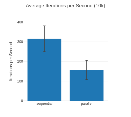
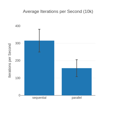
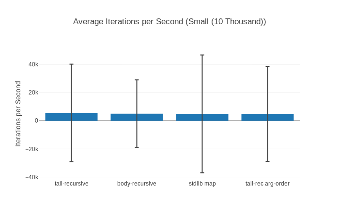
Is that the impact of the JIT you may ask? It can certainly seem so – when we’re looking at the list with 10 000 elements as input we see that even the slowest JIT implementation is faster than the fastest non-JIT implementation (remember, the JIT was introduced in OTP 24):

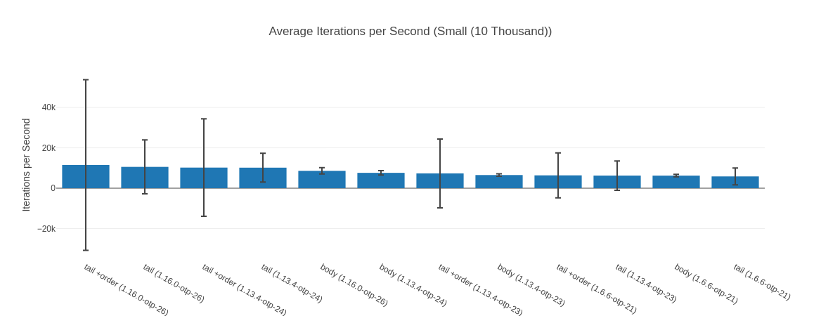
Table with more detailed data

Name	Iterations per Second	Average	Deviation	Median	Mode	Minimum	Maximum	Sample size
tail +order (1.16.0-otp-26)	11.48 K	87.10 μs	±368.22%	72.35 μs	71.78 μs	68.68 μs	200466.90 μs	457086
tail (1.16.0-otp-26)	10.56 K	94.70 μs	±126.50%	79.80 μs	79.35 μs, 79.36 μs	75.70 μs	64483.82 μs	420519
tail +order (1.13.4-otp-24)	10.20 K	98.01 μs	±236.80%	84.80 μs	81.91 μs	79.22 μs	123986.92 μs	405920
tail (1.13.4-otp-24)	10.17 K	98.37 μs	±70.24%	85.55 μs	82.62 μs	81.05 μs	41801.49 μs	404374
body (1.16.0-otp-26)	8.61 K	116.19 μs	±18.37%	118.16 μs	86.39 μs	83.71 μs	5156.24 μs	343072
body (1.13.4-otp-24)	7.60 K	131.50 μs	±13.94%	129.71 μs	125.90 μs, 125.72 μs, 125.91 μs	106.46 μs	5935.86 μs	302924
tail +order (1.13.4-otp-23)	7.34 K	136.32 μs	±232.24%	120.61 μs	109.26 μs	106.66 μs	168040.73 μs	292044
body (1.13.4-otp-23)	6.51 K	153.55 μs	±9.75%	153.70 μs	147.51 μs	139.84 μs	5164.72 μs	259470
tail +order (1.6.6-otp-21)	6.36 K	157.14 μs	±175.28%	142.99 μs	138.40 μs	122.31 μs	101605.07 μs	253459
tail (1.13.4-otp-23)	6.25 K	159.92 μs	±116.12%	154.20 μs	125.40 μs	115.74 μs	47040.19 μs	249144
body (1.6.6-otp-21)	6.23 K	160.49 μs	±9.88%	159.88 μs	159.82 μs	109.67 μs	4938.61 μs	248259
tail (1.6.6-otp-21)	5.83 K	171.54 μs	±71.94%	158.44 μs	157.72 μs	121.83 μs	40861.21 μs	232243

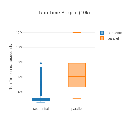
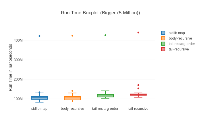
You can see the standard deviation here can be quite high, which is “thanks” to a few outliers that make the boxplot almost unreadable. Noise from Garbage Collection is often a bit of a problem with micro-benchmarks, but the results are stable and the sample size big enough. Here is a highly zoomed in boxplot to make it readable:

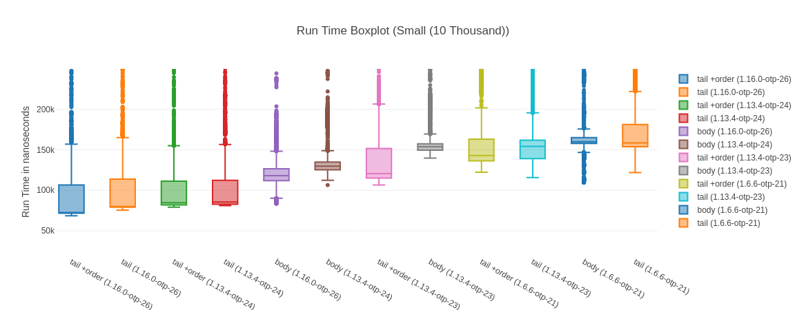
What’s really impressive to me is that the fastest version is 57% faster than the fastest non JIT version (tail +order (1.16.0-otp-26) vs. tail +order (1.13.4-otp-23)). Of course, this is a very specific benchmark and may not be indicative of overall performance gains – it’s impressive nonetheless. The other good sign is that we seem to be continuing to improve, as our current best version is 13% faster than anything available on our other most recent platform (1.13 @ OTP 24.3).

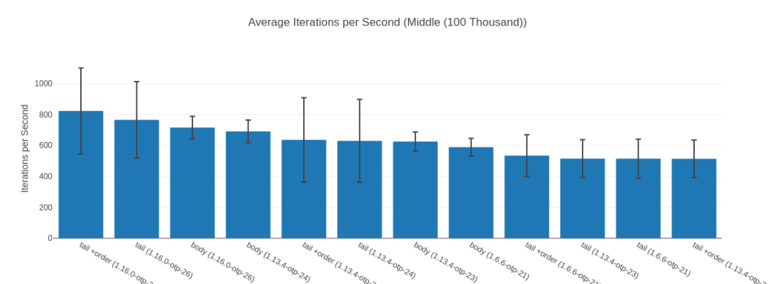
The performance uplift of Elixir 1.16 running on OTP 26.2 is even more impressive when we look at the input list of 100k elements – where all its map implementations take the 3 top spots:

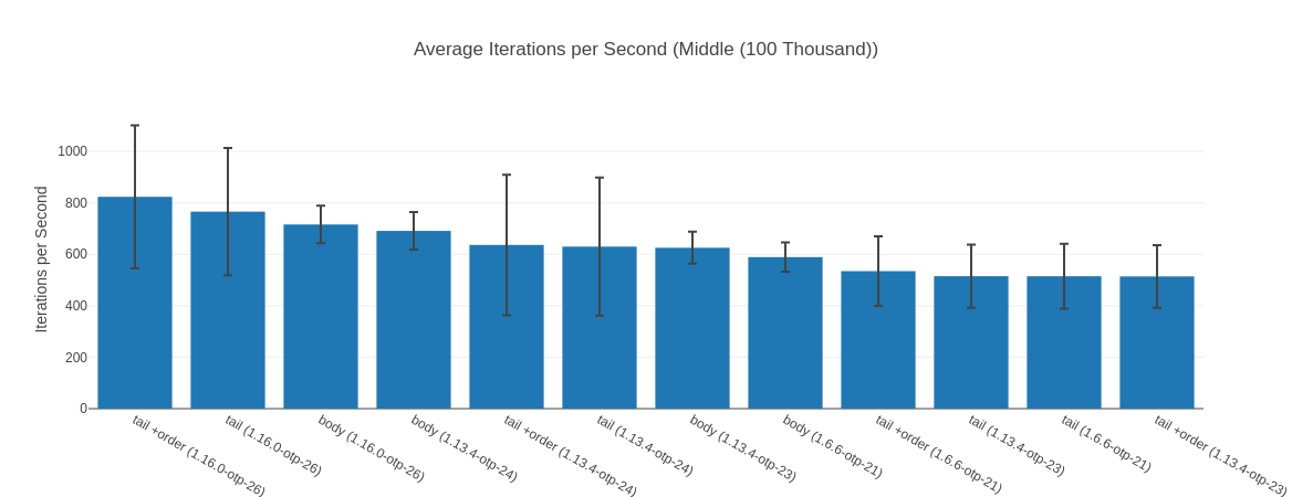
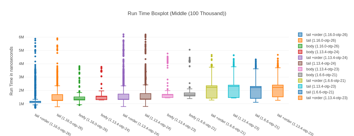
Table with more detailed data

Name	Iterations per Second	Average	Deviation	Median	Mode	Minimum	Maximum	Sample size
tail +order (1.16.0-otp-26)	823.46	1.21 ms	±33.74%	1.17 ms	0.71 ms	0.70 ms	5.88 ms	32921
tail (1.16.0-otp-26)	765.87	1.31 ms	±32.35%	1.25 ms	0.78 ms	0.77 ms	5.91 ms	30619
body (1.16.0-otp-26)	715.86	1.40 ms	±10.19%	1.35 ms	1.51 ms, 1.28 ms	0.90 ms	3.82 ms	28623
body (1.13.4-otp-24)	690.92	1.45 ms	±10.57%	1.56 ms	1.30 ms, 1.31 ms	1.29 ms	3.77 ms	27623
tail +order (1.13.4-otp-24)	636.45	1.57 ms	±42.91%	1.33 ms	1.32 ms, 1.32 ms, 1.32 ms, 1.32 ms, 1.32 ms, 1.32 ms	0.79 ms	6.21 ms	25444
tail (1.13.4-otp-24)	629.78	1.59 ms	±42.61%	1.36 ms	1.36 ms	0.80 ms	6.20 ms	25178
body (1.13.4-otp-23)	625.42	1.60 ms	±9.95%	1.68 ms	1.45 ms, 1.45 ms	1.44 ms	4.77 ms	25004
body (1.6.6-otp-21)	589.10	1.70 ms	±9.69%	1.65 ms	1.64 ms	1.39 ms	5.06 ms	23553
tail +order (1.6.6-otp-21)	534.56	1.87 ms	±25.30%	2.22 ms	1.42 ms	1.28 ms	4.67 ms	21373
tail (1.13.4-otp-23)	514.88	1.94 ms	±23.90%	2.31 ms	1.44 ms, 1.44 ms	1.43 ms	4.65 ms	20586
tail (1.6.6-otp-21)	514.64	1.94 ms	±24.51%	2.21 ms	1.40 ms	1.11 ms	4.33 ms	20577
tail +order (1.13.4-otp-23)	513.89	1.95 ms	±23.73%	2.23 ms	1.52 ms	1.26 ms	4.67 ms	20547

Here the speedup of “fastest JIT vs. fastest non JIT” is still a great 40%. Interestingly here though, for all versions except for Elixir 1.16.0 on OTP 26.2 the body-recursive functions are faster than their tail-recursive counter parts. Hold that thought for later, let’s first take a look a weird outlier – the input list with 1 Million elements.

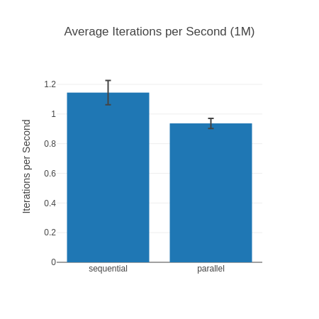
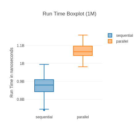
The Outlier Input – 1 Million

So, why is that the outlier? Well, here Elixir 1.13 on OTP 24.3 is faster than Elixir 1.16 on OTP 26.2! Maybe we just got unlucky you may think, but I have reproduced this result over many different runs of this benchmark. The lead also goes away again with an input list of 10 Million. Now, you may say “Tobi, we shouldn’t be dealing with lists of 1 Million and up elements anyhow” and I’d agree with you. Humor me though, as I find it fascinating what a huge impact inputs can have as well as how “random” they are. At 100k and 10 Million our Elixir 1.16 is fastest, but somehow for 1 Million it isn’t? I have no idea why, but it seems legit.

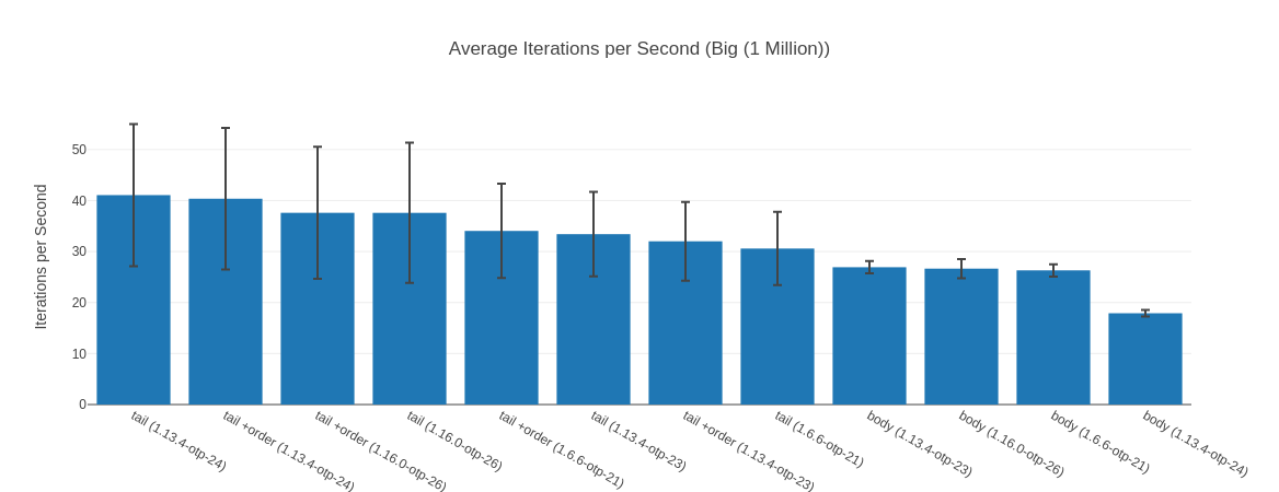
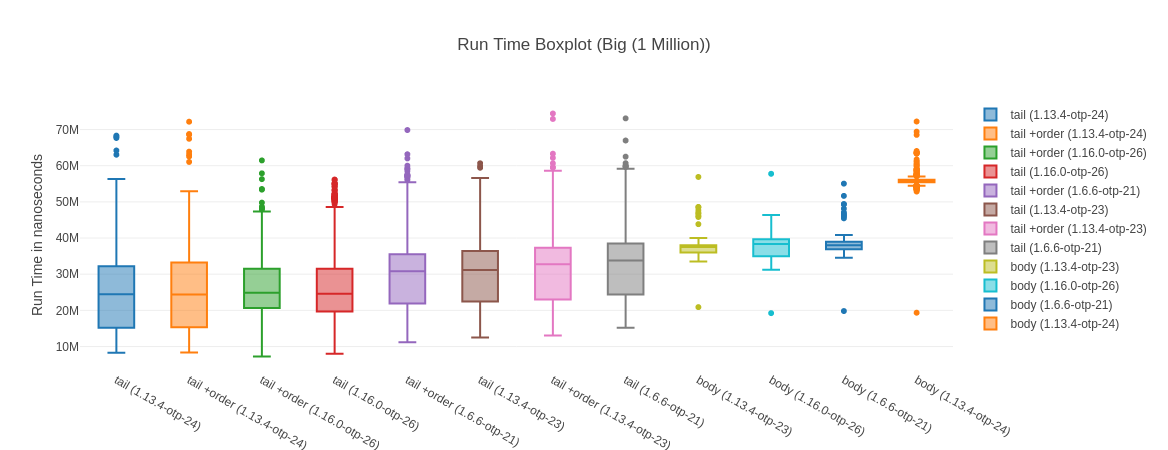
Table with more data

Name	Iterations per Second	Average	Deviation	Median	Mode	Minimum	Maximum	Sample size
tail (1.13.4-otp-24)	41.07	24.35 ms	±33.92%	24.44 ms	none	8.31 ms	68.32 ms	1643
tail +order (1.13.4-otp-24)	40.37	24.77 ms	±34.43%	24.40 ms	33.33 ms, 15.15 ms	8.36 ms	72.16 ms	1615
tail +order (1.16.0-otp-26)	37.60	26.60 ms	±34.40%	24.86 ms	26.92 ms	7.25 ms	61.46 ms	1504
tail (1.16.0-otp-26)	37.59	26.60 ms	±36.56%	24.57 ms	none	8.04 ms	56.17 ms	1503
tail +order (1.6.6-otp-21)	34.05	29.37 ms	±27.14%	30.79 ms	37.39 ms	11.20 ms	69.86 ms	1362
tail (1.13.4-otp-23)	33.41	29.93 ms	±24.80%	31.17 ms	none	12.47 ms	60.67 ms	1336
tail +order (1.13.4-otp-23)	32.01	31.24 ms	±24.13%	32.78 ms	23.27 ms	13.06 ms	74.43 ms	1280
tail (1.6.6-otp-21)	30.59	32.69 ms	±23.49%	33.78 ms	none	15.17 ms	73.09 ms	1224
body (1.13.4-otp-23)	26.93	37.13 ms	±4.54%	37.51 ms	38.11 ms	20.90 ms	56.89 ms	1077
body (1.16.0-otp-26)	26.65	37.52 ms	±7.09%	38.36 ms	none	19.23 ms	57.76 ms	1066
body (1.6.6-otp-21)	26.32	38.00 ms	±4.56%	38.02 ms	none	19.81 ms	55.04 ms	1052
body (1.13.4-otp-24)	17.90	55.86 ms	±3.63%	55.74 ms	none	19.36 ms	72.21 ms	716

Before we dig in, it’s interesting to notice that at the 1 Million inputs mark, the body-recursive functions together occupy the last 4 spots of our ranking. It stays like this for all bigger inputs.

When I look at a result that is “weird” to me I usually look at a bunch of other statistical values: 99th%, median, standard deviation, maximum etc. to see if maybe there were some weird outliers here. Specifically I’m checking whether the medians roughly line up with the averages in their ordering – which they do here. Everything seems fine here.

The next thing I’m looking are the raw recorded run times (in order) as well as their general distribution. While looking at those you can notice some interesting behavior. While both elixir 1.13 @ OTP 24.3 solutions have a more or less steady pattern to their run times, their elixir 1.16 @ OTP 26.2 counter parts seem to experience a noticeable slow down towards the last ~15% of their measurement time. Let’s look at 2 examples for the the tail +order variants:

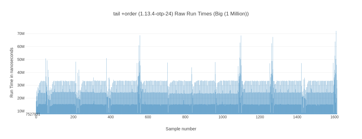
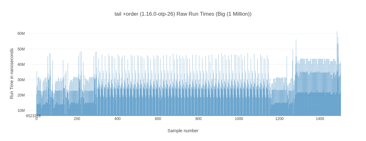
Why is this happening? I don’t know – you could blame it on on some background job or something kicking in but then it wouldn’t be consistent across tail and tail +order for the elixir 1.16 variant. While we’re looking at these graphs, what about the bod-recursive cousin?

Less Deviation for Body-Recursive Functions

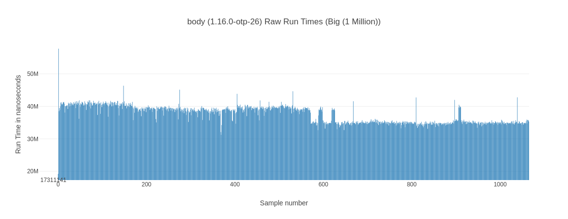
The body-recursive version looks a lot smoother and less jittery. This is something you can observe across all inputs – as indicated by the much lower standard-deviation of body-recursive implementations.

Memory Consumption

The memory consumption story is much less interesting – body-recursive functions consume less memory and by quite the margin! ~50% of the tail-recursive functions for all but our smallest input size – there it’s still 70%.

This might also be one of the key to seeing less jittery run times – less memory means less garbage produced means fewer garbage collection runs necessary.

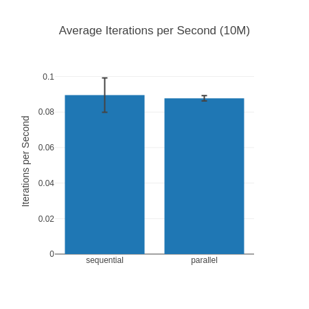
A 60%+ lead – the 10 Million Input

What I found interesting looking at the results is that for our 10 Million input elixir 1.16 @ OTP 26 is 67% faster than the next fastest implementation. Which is a huge difference.

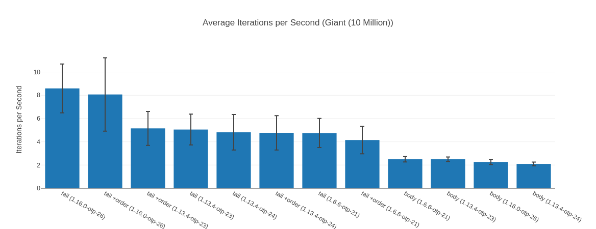
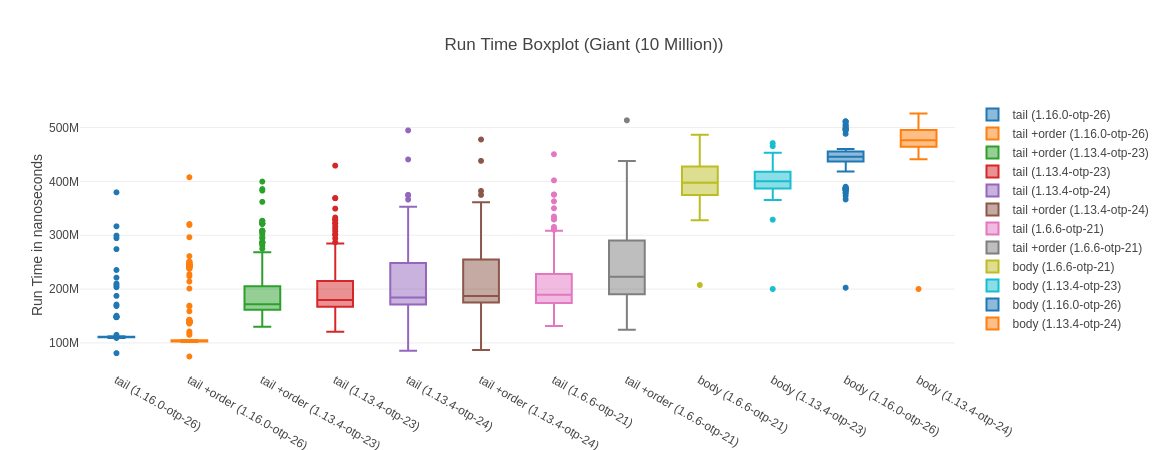
Table with more data

Name	Iterations per Second	Average	Deviation	Median	Mode	Minimum	Maximum	Sample size
tail (1.16.0-otp-26)	8.59	116.36 ms	±24.44%	111.06 ms	none	81.09 ms	379.73 ms	343
tail +order (1.16.0-otp-26)	8.07	123.89 ms	±39.11%	103.42 ms	none	74.87 ms	407.68 ms	322
tail +order (1.13.4-otp-23)	5.15	194.07 ms	±28.32%	171.83 ms	none	129.96 ms	399.67 ms	206
tail (1.13.4-otp-23)	5.05	197.91 ms	±26.21%	179.95 ms	none	120.60 ms	429.31 ms	203
tail (1.13.4-otp-24)	4.82	207.47 ms	±31.62%	184.35 ms	none	85.42 ms	494.75 ms	193
tail +order (1.13.4-otp-24)	4.77	209.59 ms	±31.01%	187.04 ms	none	86.99 ms	477.82 ms	191
tail (1.6.6-otp-21)	4.76	210.30 ms	±26.31%	189.71 ms	224.04 ms	131.60 ms	450.47 ms	190
tail +order (1.6.6-otp-21)	4.15	240.89 ms	±28.46%	222.87 ms	none	124.69 ms	513.50 ms	166
body (1.6.6-otp-21)	2.50	399.78 ms	±9.42%	397.69 ms	none	207.61 ms	486.65 ms	100
body (1.13.4-otp-23)	2.50	399.88 ms	±7.58%	400.23 ms	none	200.16 ms	471.13 ms	100
body (1.16.0-otp-26)	2.27	440.73 ms	±9.60%	445.77 ms	none	202.63 ms	511.66 ms	91
body (1.13.4-otp-24)	2.10	476.77 ms	±7.72%	476.57 ms	none	200.17 ms	526.09 ms	84

We also see that the tail-recursive solution here is almost 4 times as fast as the body-recursive version. Somewhat interestingly the version without the argument order switch seems faster here (but not by much). You can also see that the median is (considerably) in favor of tail +order against its just tail counter part.

Let’s take another look at our new found friend – the raw run times chart:

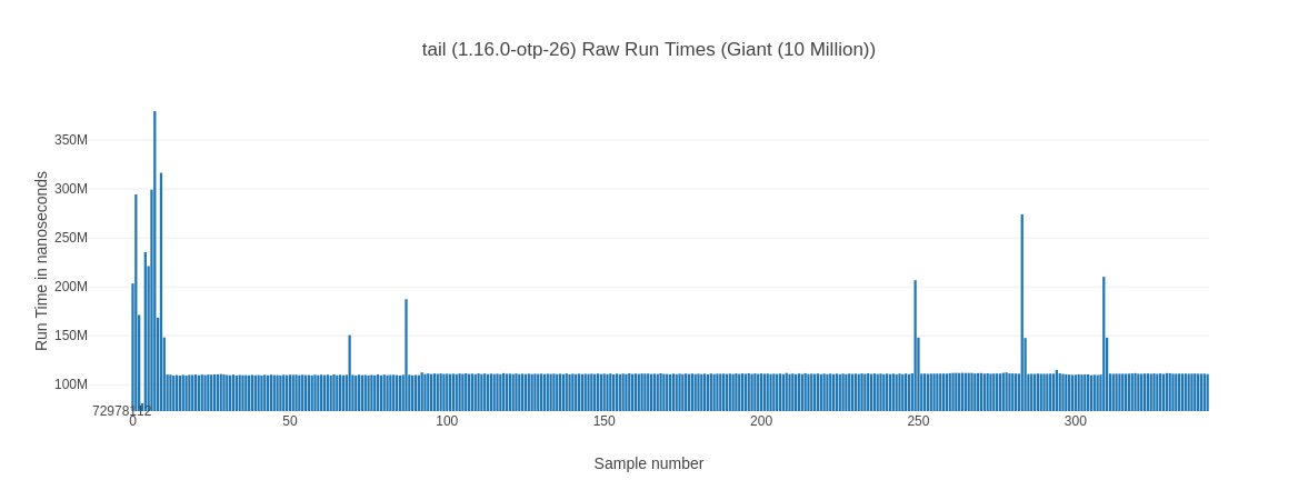
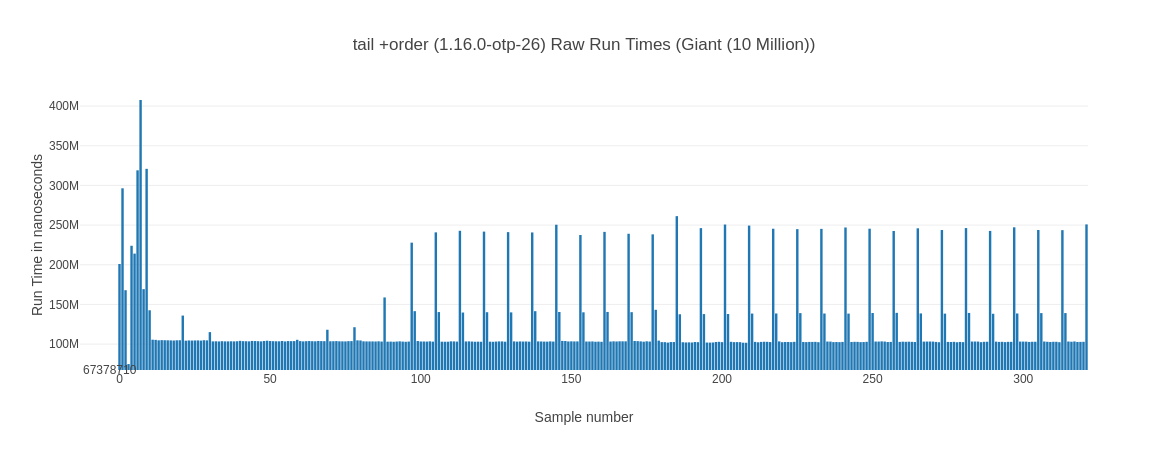
We can clearly see that the tail +order version goes into a repeating pattern of taking much longer every couple of runs while the tail version is (mostly) stable. That explains the lower average while it has a higher median for the tail version. It is faster on average by being more consistent – so while its median is slightly worse it is on average faster as it doesn’t exhibit these spikes. Why is this happening? I don’t know, except that I know I’ve seen it more than once.

The body-recursive to tail-recursive reversal

As you may remember from the intro, this journey once began with “Tail Call Optimization in Elixir & Erlang – not as efficient and important as you probably think” – claiming that body-recursive version was faster than the tail-recursive version. The last revision showed some difference in what function was faster based on what input was used.

And now? For Elixir 1.16 on OTP 26.2 the tail-recursive functions are faster than their body-recursive counter part on all tested inputs! How different depends on the input size – from just 15% to almost 400% we’ve seen it all.

This is also a “fairly recent” development – for instance for our 100k input for Elixir 1.13@OTP 24 the body-recursive function is the fastest.

Naturally that still doesn’t mean everything should be tail-recursive: This is one benchmark with list sizes you may rarely see. Memory consumption and variance are also points to consider. Also let’s remember a quote from “The Seven Myths of Erlang Performance” about this:

It is generally not possible to predict whether the tail-recursive or the body-recursive version will be faster. Therefore, use the version that makes your code cleaner (hint: it is usually the body-recursive version).

And of course, some use cases absolutely need a tail-recursive function (such as Genservers).

Finishing Up

So, what have we discovered? On our newest Elixir and Erlang versions tail-recursive functions shine more than they did before – outperforming the competition. We have seen some impressive performance improvements over time, presumably thanks to the JIT – and we seem to be getting even more performance improvements.

As always, run your own benchmarks – don’t trust some old post on the Internet saying one thing is faster than another. Your compiler, your run time – things may have changed.

Lastly, I’m happy to finally publish these results – it’s been a bit of a yak shave. But, a fun one! 😁

Careful what data you send or how to tank your performance with Task.async

In Elixir and on the BEAM (Erlang Virtual Machine) in general we love our processes – lightweight, easily run millions of them, easy lock-less parallelism – you’ve probably heard it all. Processes are great and one of the many reasons people gravitate towards the BEAM.

Functions like Task.async/1 make parallelism effortless and can feel almost magical. Cool, let’s use it in a simple benchmark! Let’s create some random lists, and then let’s run some non trivial Enum functions on them: uniq, frequencies and shuffle and let’s compare doing them sequentially (one after the other) and running them all in parallel. This kind of work is super easy to parallelize, so we can just fire off the tasks and then await them:

	random_list = fn size, spread ->
	for _i <- 1..size, do: :rand.uniform(spread)
	end
	inputs = [
	{"10k", random_list.(10_000, 100)},
	{"1M", random_list.(1_000_000, 1_000)},
	{"10M", random_list.(10_000_000, 10_000)}
	]
	Benchee.run(
	%{
	"sequential" => fn big_list ->
	uniques = Enum.uniq(big_list)
	frequencies = Enum.frequencies(big_list)
	shuffled = Enum.shuffle(big_list)
	[uniques, frequencies, shuffled]
	end,
	"parallel" => fn big_list ->
	tasks = [
	Task.async(fn -> Enum.uniq(big_list) end),
	Task.async(fn -> Enum.frequencies(big_list) end),
	Task.async(fn -> Enum.shuffle(big_list) end)
	]
	Task.await_many(tasks, :infinity)
	end
	},
	inputs: inputs,
	warmup: 15,
	time: 60,
	formatters: [
	{Benchee.Formatters.Console, extended_statistics: true},
	{Benchee.Formatters.HTML, file: "bench/output/task_no_task/index.html", auto_open: false}
	]
	)

view raw benchmark.exs hosted with ❤ by GitHub

Cool, let’s check out the results! You can check the HTML report online here, uncollapse for the console formatter version or just check out the pictures.

Console formatter output

Operating System: Linux
CPU Information: AMD Ryzen 9 5900X 12-Core Processor
Number of Available Cores: 24
Available memory: 31.25 GB
Elixir 1.16.0-rc.1
Erlang 26.1.2
JIT enabled: true

Benchmark suite executing with the following configuration:
warmup: 15 s
time: 1 min
memory time: 0 ns
reduction time: 0 ns
parallel: 1
inputs: 10k, 1M, 10M
Estimated total run time: 7.50 min

##### With input 10k #####
Name                 ips        average  deviation         median         99th %
sequential        315.29        3.17 ms    ±20.76%        2.96 ms        5.44 ms
parallel          156.77        6.38 ms    ±31.08%        6.11 ms       10.75 ms

Comparison: 
sequential        315.29
parallel          156.77 - 2.01x slower +3.21 ms

Extended statistics: 

Name               minimum        maximum    sample size                     mode
sequential         2.61 ms        7.84 ms        18.91 K         2.73 ms, 3.01 ms
parallel           3.14 ms       11.99 ms         9.40 K4.80 ms, 4.87 ms, 8.93 ms

##### With input 1M #####
Name                 ips        average  deviation         median         99th %
sequential          1.14         0.87 s     ±7.16%         0.88 s         0.99 s
parallel            0.94         1.07 s     ±3.65%         1.07 s         1.16 s

Comparison: 
sequential          1.14
parallel            0.94 - 1.22x slower +0.194 s

Extended statistics: 

Name               minimum        maximum    sample size                     mode
sequential          0.74 s         0.99 s             69                     None
parallel            0.98 s         1.16 s             57                     None

##### With input 10M #####
Name                 ips        average  deviation         median         99th %
sequential        0.0896        11.17 s    ±10.79%        11.21 s        12.93 s
parallel          0.0877        11.40 s     ±1.70%        11.37 s        11.66 s

Comparison: 
sequential        0.0896
parallel          0.0877 - 1.02x slower +0.23 s

Extended statistics: 

Name               minimum        maximum    sample size                     mode
sequential          9.22 s        12.93 s              6                     None
parallel           11.16 s        11.66 s              6                     None

10k input, iterations per second (higher is better)

Boxplot for 10k, measured run time (lower is better). Sort of interesting how many “outliers” (blue dots) there are for sequential though.

1M input, iterations per second (higher is better)

Boxplot for 1M, measured run time (lower is better).

10M input, iterations per second (higher is better). Important to know, they take so long here the sample size is only 6 for each.

And just as we all expected the parallel… no wait a second the sequential version is faster for all of them? How could that be? This was easily parallelizable work, split into 3 work packages with many more cores available to do the work. Why is the parallel execution slower?

What happened here?

There’s no weird trick to this: It ran on a system with 12 physical cores that was idling save for the benchmark. Starting processes is extremely fast and lightweight, so that’s also not it. By most accounts, parallel processing should win out.

What is the problem then?

The problem here are the huge lists the tasks need to operate on and the return values that need to get back to the main process. The BEAM works on a “share nothing” architecture, this means in order to process theses lists in parallel we have to copy the lists over entirely to the process (Tasks are backed by processes). And once they’re done, we need to copy over the result as well. Copying, esp. big data structures, is both CPU intensive and memory intensive. In this case the additional copying work we do outweighs the gains we get by processing the data in parallel. You can also see that this effect seems to be diminishing the bigger the lists get – so it seems like the parallelization is catching up there.

The full copy may sound strange – after all we’re dealing with immutable data structures which should be safe to share. Well, once processes share data garbage collection becomes a whole other world of complex, or in the words of the OTP team in “A few notes on message passing” (emphasis mine):

Sending a message is straightforward: we try to find the process associated with the process identifier, and if one exists we insert the message into its signal queue.

Messages are always copied before being inserted into the queue. As wasteful as this may sound it greatly reduces garbage collection (GC) latency as the GC never has to look beyond a single process. Non-copying implementations have been tried in the past, but they turned out to be a bad fit as low latency is more important than sheer throughput for the kind of soft-realtime systems that Erlang is designed to build.

John Högberg

Robert Virding (co-inventor of Erlang) also puts some more color to it in a thread on elixir forum.

In case you’re interested in other factors for this particular benchmark: I chose the 3 functions semi-randomly looking for functions that traverse the full list at least once doing some non trivial work. If you do heavier work on the lists the parallel solution will fare better. We can also not completely discount that CPU boosting (where single core performance may increase if the other cores are idle) is shifting benchmark a bit in favor of sequential but overall it should be solid enough for demonstration purposes. Due to the low sample size for the 10M list, parallel execution may sometimes come out ahead, but usually doesn’t (and I didn’t want the benchmark take even longer).

The Sneakyness

Now, the problem here is a bit more sneaky – as we’re not explicitly sending messages. Our code looks like this: Task.async(fn -> Enum.uniq(big_list) end) – there is no send or GenServer.call here! However, that function still needs to make its way to the process for execution. As the closure of the function automatically captures referenced variables – all that data ends up being copied over as well! (Technically speaking Task.async does a send under the hood, but spawn/1 also behaves like this.)

This is what caught me off-guard with this – I knew messages were copied, but somehow Task.async was so magical I didn’t think about it sending messages or needing to copy its data to a process. Let’s call it a blind spot and broken mental model I’ve had for way too long. Hence, this blog post is for you dear reader – may you avoid the mistake I made!

Let’s also be clear here that normally this isn’t a problem and the benefits we get from this behavior are worth it. When a process terminates we can just free all its memory. It’s also not super common to shift so much data to a process to do comparatively lightweight work. The problem here is a bit, how easy it is for this problem to sneak up on you when using these high level abstractions like Task.async/1.

Real library, real problems

Yup. While I feel some shame about it, I’ve always been an advocate for sharing mistakes you made to spread some of the best leanings. This isn’t a purely theoretical thing I ran into – it stems from real problems I encountered. As you may know I’m the author of benchee – the best benchmarking library ™ 😉 . Benchee’s design, in a nut shell, revolves around a big data structure – the suite – data is enriched throughout the process of benchmarking. You may get a better idea by looking at the breakdown of the steps. This has worked great for us.

However, some of the data in that suite may reference large chunks of data if the benchmark operates on large data. Each Scenario references its given input as well as its benchmarking function. Given what we just learned both of these may be huge. More than that, the Configuration also holds all the configured inputs and is part of the suite as well.

Now, when benchee tries to compute your statistics in parallel it happily creates a new process for each scenario (which may be 20+) copying over the benchmarking function and input although it really doesn’t need them.

Even worse formatters are run in parallel handing over the entire suite – including all scenarios (function and input) as well as all the inputs again as part of the Configuration – none of which a formatter should need. 😱

To be clear, you will only encounter this problem if you deal with huge sets of data and if you do it’s “just” more memory and time used. However, for a library about measuring things and making them fast this is no good.

The remedy

Thankfully, there are multiple possible remedies for this problem:

• Limiting the data you send to the absolute necessary minimum, instead of just sending the whole struct. For example, don’t send an entire Suite struct if all you need is a couple of fields.
• If only the process needs the data, it may fetch the data itself instead. I.e. instead of putting the result of a giant query into the process, the process could be the one doing the query if it’s the only one that needs the data.
• There are some data structures that are shared between processes and hence don’t need copying, such as ets and persistent_term.

As teased above, the most common and easiest solution is just to pass along the data you need, if you ended up accidentally sending along more than you wanted to. You can see one step of it in this pull request or this one.

The results are quite astounding, for a benchmark I’m working on (blog post coming soon ™) this change got it from practically being unable to run the benchmark due to memory constraints (on a 32GB RAM system) to easily running the benchmark – maximum resident size set size got almost halfed.

The magnitude of this can also be shown perhaps by the size of the files I saved for this benchmark. Saving is actually implemented as a formatter, and so automatically benefits from these changes – the file size for this benchmark went down from ~200MB per file to 1MB aka a reduction to 0.5% in size. You can read more about how it improved in the benchee 1.3.0 release notes.

Naturally this change will also make its way to you all as benchee 1.3.0 soon (edit: out now!).

Also when pursuing to fix this be mindful that you need to completely remove the variable from the closure. You can’t just go: Task.async(fn -> magic(suite.configuration) end) – the entire suite will still be sent along.

iex(1)> list = Enum.to_list(1..100_000)
iex(2)> # do not benchmark in iex, this is purely done to get a suite with some data
iex(3)> suite = Benchee.run(%{map: fn -> Enum.map(list, fn i -> i * i end) end })
iex(4)> :erts_debug.size(suite)
200642
iex(5)> :erts_debug.size(fn -> suite end)
200675
iex(6)> :erts_debug.size(fn -> suite.configuration end)
200841
iex(7)> :erts_debug.size(fn -> suite.configuration.time end)
201007
iex(8)> configuration = suite.configuration
iex(9)> :erts_debug.size(fn -> configuration.time end)
295
iex(10)> time = configuration.time
iex(11)> :erts_debug.size(fn -> time end)
54

Helping others avoid making the same mistake

All of that discovery, and partially shame, left me with the question: How can I help others avoid making the same mistake? Well, one part of it is right here – publish a blog post. However, that’s one point.

We already added documentation to the Task module mentioning this, and as proposed by José are working on adding a section to the process anti-patterns section.

Also don’t forget: processes are still awesome and lightweight – you should use them! This is just a cautionary tale of how things might go wrong if you’re dealing with big chunks of data and that the work you’re doing on that data may not be extensive enough to warrant a full copy. Or that you’re accidentally sending along too much data unaware of the consequences. There are many more use cases for processes and tasks that are absolutely great, appropriate and will save you a ton of time.

What does this leave us with? As usual: don’t assume, always benchmark!

Also, be careful about the data you’re sending around and if you really need it! 💚

The great Rubykon Benchmark 2020: CRuby vs JRuby vs TruffleRuby

It has been far too long, more than 3.5 years since the last edition of this benchmark. Well what to say? I almost had a new edition ready a year ago and then the job hunt got too intense and now the heat wave in Berlin delayed me. You don’t want your computer running at max capacity for an extended period, trust me.

Well, you aren’t here to hear about why there hasn’t been a new edition in so long, you’re here to read about the new edition! Most likely you’re here to look at graphs and see what’s the fastest ruby implementation out there. And I swear we’ll get to it but there’s some context to establish first. Of course, feel free to skip ahead if you just want the numbers.

Well, let’s do this!

What are we benchmarking?

We’re benchmarking Rubykon again, a Go AI written in Ruby using Monte Carlo Tree Search. It’s a fun project I wrote a couple of years back. Basically it does random playouts of Go games and sees what moves lead to a winning game building a tree with different game states and their win percentages to select the best move.

Why is this a good problem to benchmark? Performance matters. The more playouts we can do the better our AI plays because we have more data for our decisions. The benchmark we’re running starts its search from an empty 19×19 board (biggest “normal” board) and does 1000 full random playouts from there. We’ll measure how long that takes/how often we could do that in a minute. This also isn’t a micro benchmark, while remaining reasonable in size it looks at lots of different methods and access patterns.

Why is this a bad problem to benchmark? Most Ruby devs are probably interested in some kind of web application performance. This does no IO (which keeps the focus on ruby code execution, which is also good) and mainly deals with arrays. While we deal with collections all the time, rubykon also accesses a lot of array indexes all over, which isn’t really that common. It also barely deals with strings. Moreover, it does a whole lot of (pseudo-)random number generation which definitely isn’t a common occurrence. It also runs a relatively tight hot loop of “generate random valid move, play it, repeat until game over”, which should be friendly to JIT approaches.

What I want to say, this is an interesting problem to benchmark but it’s probably not representative of web application performance of the different ruby implementations. It is still a good indicator of where different ruby implementations rank performance wise.

It’s also important to note that this benchmark is single threaded – while it is a problem suited for parallelization I haven’t done so yet. Plus, single threaded applications are still typical for Ruby (due to the global interpreter lock in CRuby).

We’re also mainly interested in “warm” application performance i.e. giving them a bit of time to warm up and look at their peak performance. We’ll also look at the warmup times in a separate section though.

The competitors

Our competitors are ruby variants I could easily install on my machine and was interested in which brings us to:

• CRuby 2.4.10
• CRuby 2.5.8
• CRuby 2.6.6
• CRuby 2.7.1
• CRuby 2.8.0-dev (b4b702dd4f from 2020-08-07) (this might end up being called Ruby 3 not 2.8)
• truffleruby-1.0.0-rc16
• truffleruby-20.1.0
• jruby-9.1.17.0
• jruby-9.2.11.1

All of those versions were current as of early August 2020. As usual doing all the benchmarking, graphing and writing has taken me some time so that truffleruby released a new version in the mean time, result shouldn’t differ much though.

CRuby (yes I still insist on calling it that vs. MRI) is mainly our base line as it’s the standard ruby interpreter. Versions that are capable of JITing (2.6+) will also be run with the –jit flag separately to show improvement (also referred to as MJIT).

TruffleRuby was our winner the last 2 times around. We’re running 20.1 and 1.0-rc16 (please don’t ask me why this specific version, it was in the matrix from when I originally redid this benchmarks a year ago). We’re also going to run both native and JVM mode for 20.1.

JRuby will be run “normally”, and with invokedynamic + server flag (denoted by “+ID”). We’re also gonna take a look at JDK 8 and JDK 14. For JDK 14 we’re also going to run it with a non default GC algorithm, falling back to the one used in JDK 8 as the new default is slower for this benchmark. Originally I also wanted to run with lots of different JVMs but as it stands I already recorded almost 40 different runs in total and the JVMs I tried didn’t show great differences so we’ll stick with the top performer of those I tried which is AdoptOpenJDK.

You can check all flags passed etc. in the benchmark script.

The Execution Environment

This is still running on the same Desktop PC that I did the first version of these benchmarks with – almost 5 years ago. In the meantime it was hit by a lot of those lovely intel security vulnerabilities though. It’s by no means a top machine any more.

The machine has 16 GB of RAM, runs Linux Mint 19.3 (based on Ubuntu 18.04 LTS) and most importantly an i7-4790 (3.6 GHz, 4 GHz boost) (which is more than 6 years old now).

	tobi@speedy:~$ uname -a
	Linux speedy 5.4.0-42-generic #46~18.04.1-Ubuntu SMP Fri Jul 10 07:21:24 UTC 2020 x86_64 x86_64 x86_64 GNU/Linux
	tobi@speedy:~$ lscpu
	Architecture: x86_64
	CPU op-mode(s): 32-bit, 64-bit
	Byte Order: Little Endian
	CPU(s): 8
	On-line CPU(s) list: 0-7
	Thread(s) per core: 2
	Core(s) per socket: 4
	Socket(s): 1
	NUMA node(s): 1
	Vendor ID: GenuineIntel
	CPU family: 6
	Model: 60
	Model name: Intel(R) Core(TM) i7-4790 CPU @ 3.60GHz
	Stepping: 3
	CPU MHz: 3568.176
	CPU max MHz: 4000,0000
	CPU min MHz: 800,0000
	BogoMIPS: 7200.47
	Virtualization: VT-x
	L1d cache: 32K
	L1i cache: 32K
	L2 cache: 256K
	L3 cache: 8192K
	NUMA node0 CPU(s): 0-7
	Flags: fpu vme de pse tsc msr pae mce cx8 apic sep mtrr pge mca cmov pat pse36 clflush dts acpi mmx fxsr sse sse2 ss ht tm pbe syscall nx pdpe1gb rdtscp lm constant_tsc arch_perfmon pebs bts rep_good nopl xtopology nonstop_tsc cpuid aperfmperf pni pclmulqdq dtes64 monitor ds_cpl vmx smx est tm2 ssse3 sdbg fma cx16 xtpr pdcm pcid sse4_1 sse4_2 x2apic movbe popcnt tsc_deadline_timer aes xsave avx f16c rdrand lahf_lm abm cpuid_fault epb invpcid_single pti ssbd ibrs ibpb stibp tpr_shadow vnmi flexpriority ept vpid ept_ad fsgsbase tsc_adjust bmi1 avx2 smep bmi2 erms invpcid xsaveopt dtherm ida arat pln pts md_clear flush_l1d

view raw system_info hosted with ❤ by GitHub

All background applications were closed and while the benchmarks were running no GUI was active. They were run on hot Berlin evenings 😉

If you want to run these benchmarks yourself the rubykon repo has the instructions, with most of it being automated.

Timing wise I chose 5 minutes of warmup and 2 minutes of run time measurements. The (enormous) warmup time was mostly driven by behaviour observed in TruffleRuby where sometimes it would deoptimize even after a long warmup. So, I wanted to make sure everyone had all the time they needed to reach good “warm” performance.

Run Time Results

One more thing before we get to it: JRuby here ran on AdoptOpenJDK 8. Differences to AdoptOpenJDK 14 (and other JVMs) aren’t too big and would just clutter the graphs. We’ll take a brief look at them later.

If you want to take a look at all the data I gathered you can access the spreadsheet.

Iterations per Minute per Ruby implementation for running 1000 full playouts on a 19×19 board (higher is better).

Overall this looks more or less like the graphs from the last years:

• CRuby is the baseline performance without any major jumps
• JRuby with invokedynamic (+ID) gets a bit more than 2x the baseline performance of CRuby, invokedynamic itself makes it a lot faster (2x+)
• TruffleRuby runs away with the win

What’s new though is the inclusion of the JIT option for CRuby which performs quite impressively and is only getting better. An 18% improvement on 2.6 goes up to 34% on 2.7 and tops out at 47% for 2.8 dev when looking at the JIT vs. non JIT run times of the same Ruby version. Looking at CRuby it’s also interesting that this time around “newer” CRuby performance is largely on par with not JITed JRuby performance.

The other thing that sticks out quite hugely are those big error bars on TruffleRuby 20. This is caused by some deoptimizations even after the long warmup. Portrayed here is a run where they weren’t as bad, even if they are worse performance was still top notch at 27 i/min overall though. It’s most likely a bug that these deoptimizations happen, you can check the corresponding issue. In the past the TruffleRuby always found a way to fix issues like this. So, the theoretical performance is a bit higher.

Another thing I like to look at is the relative speedup chart:

Speedup relative to CRuby 2.4.10 (baseline)

CRuby 2.4.10 was chosen as the “baseline” for this relative speedup chart mostly as a homage to Ruby 3×3 in which the goal was for Ruby 3 to be 3 times faster than Ruby 2.0. I can’t get Ruby < 2.4 to compile on my system easily any more and hence they are sadly missing here.

I’m pretty impressed with the JIT in Ruby 2.8: a speedup of over 60% is not to be scoffed at! So, as pointed out in the results above, I have ever rising hopes for it! JRuby (with invokedynamic) sits nice and comfortably at ~2.5x speedup which is a bit down from its 3x speedup in the older benchmarks. This might also be to the improved baseline of CRuby 2.4.10 versus the old CRuby 2.0 (check the old blog post for some numbers from then, not directly comparable though). TruffleRuby sits at the top thanks to the –jvm version with almost a 6x improvement. Perhaps more impressively it’s still 2.3 times faster than the fastest non TruffleRuby implementation. The difference between “native” and –jvm for TruffleRuby is also astounding and important to keep in mind should you do your own benchmarks.

What’s a bit baffling is that the performance trend for CRuby isn’t “always getting better” like I’m used to. The differences are rather small but looking at the small standard deviation (at most less than 1%) I’m rather sure of them. 2.5 is slower than 2.4, and 2.6 is faster than both 2.7 and 2.8.-dev. However, the “proper” order is established again when enabling the JIT.

If you’re rather interested in the data table you can still check out the spreadsheet for the full data, but here’s some of it inline:

Ruby	i/min	avg (s)	stddev %	relative speedup
2.4.10	5.61	10.69	0.86	1
2.5.8	5.16	11.63	0.27	0.919786096256684
2.6.6	6.61	9.08	0.42	1.17825311942959
2.6.6 –jit	7.8	7.69	0.59	1.3903743315508
2.7.1	6.45	9.3	0.25	1.14973262032086
2.7.1 –jit	8.64	6.95	0.29	1.54010695187166
2.8.0-dev	6.28	9.56	0.32	1.11942959001783
2.8.0-dev –jit	9.25	6.48	0.29	1.64884135472371
truffleruby-1.0.0-rc16	16.55	3.63	2.19	2.95008912655971
truffleruby-20.1.0	20.22	2.97	25.82	3.60427807486631
truffleruby-20.1.0 –jvm	33.32	1.8	19.01	5.93939393939394
jruby-9.1.17.0	6.52	9.21	0.63	1.16221033868093
jruby-9.1.17.0 +ID	14.27	4.2	0.29	2.54367201426025
jruby-9.2.11.1	6.33	9.49	0.54	1.1283422459893
jruby-9.2.11.1 +ID	13.85	4.33	0.44	2.46880570409982

Warmup

Seems the JITing approaches are winning throughout, however such performance isn’t free. Conceptually, a JIT looks at what parts of your code are run often and then tries to further optimize (and often specialize) these parts of the code. This makes it a whole lot faster, this process takes time and work though.

The benchmarking numbers presented above completely ignore the startup and warmup time. The common argument for this is that in long lived applications (like most web applications) we spend the majority of time in the warmed up/hot state. It’s different when talking about scripts we run as a one off. I visualized and described the different times to measure way more in another post.

Anyhow, lets get a better feeling for those warmup times, shall we? One of my favourite methods for doing so is graphing the first couple of run times as recorded (those are all during the warmup phase):

Run times as recorded by iteration number for a few select Ruby implementations. Lower is faster/better.

Same data as above but as a line chart. Thanks to Stefan Marr for nudging me.

CRuby itself (without –jit) performs at a steady space, this is expected as no further optimizations are done and there’s also no cache or anything involved. Your first run is pretty much gonna be as fast as your last run. It’s impressive to see though that the –jit option is faster already in the first iteration and still getting better. What you can’t see in the graph, as it doesn’t contain enough run times and the difference is very small, is that the CRuby –jit option only reaches its peak performance around iteration 19 (going from ~6.7s to ~6.5s) which is quite surprising looking at how steady it seems before that.

TruffleRuby behaves in line with previous results. It has by far the longest warmup time, especially the JVM configuration which is in line with their presented pros and cons. The –jvm runtime configuration only becomes the fastest implementation by iteration 13! Then it’s faster by quite a bit though. It’s also noteworthy that for neither native nor JVM the time declines steadily. Sometimes subsequent iterations are slower which is likely due to the JIT trying hard to optimize something or having to deoptimize something. The random nature of Rubykon might play into this, as we might be hitting edge cases only at iteration 8 or so. While especially the first run time can be quite surprising, it’s noteworthy that during my years of doing these benchmarks I’ve seen TruffleRuby steadily improve its warmup time. As a datapoint, TruffleRuby 1.0.0-rc16 had its first 2 run times at 52 seconds and 25 seconds.

JRuby is very close to peak performance after one iteration already. Peak performance with invokedynamic is hit around iteration 7. It’s noteworthy that with invokedynamic even the first iteration is faster than CRuby “normal” and on par with the CRuby JIT implementation but in subsequent iterations gets much faster than them. The non invokedynamic version is very close to normal CRuby 2.8.0-dev performance almost the entire time, except for being slower in the first iteration.

For context it’s important to point out though that Rubykon is a relatively small application. Including the benchmarking library it’s not even 1200 lines of code long. It uses no external gems, it doesn’t even access the standard library. So all of the code is in these 1200 lines + the core Ruby classes (Array etc.) which is a far cry from a full blown Rails application. More code means more things to optimize and hence should lead to much longer warmup times than presented here.

JRuby/JVM musings

It might appear unfair that the results up there were run only with JDK 8. I can assure you, in my testing it sadly isn’t. I had hoped for some big performance jumps with the new JDK versions but I found no such thing. Indeed, it features the fastest version but only by a rather slim margin. It also requires switching up the GC algorithm as the new default performs worse at least for this benchmark.

Comparison JRuby with different options against AdoptOpenJDK 8 and 14

Performance is largely the same. JDK 14 is a bit faster when using both invokedynamic and falling back to the old garbage collector (+ParallelGC). Otherwise performance is worse. You can find out more in this issue. It’s curios though that JRuby 9.1 seems mostly faster than 9.2.

I got also quite excited at first looking at all the different new JVMs and thought I’d benchmark against them all, but it quickly became apparent that this was a typical case of “matrix explosion” and I really wanted for you all to also see these results unlike last year 😅 I gathered data for GraalVM and Java Standard Edition Reference Implementation in addition to AdoptOpenJDK but performance was largely the same and best at AdoptOpenJDK on my system for this benchmark. Again, these are in the spreadsheet.

I did one more try with OpenJ9 as it sounded promising. The results were so bad I didn’t even put them into the spreadsheet (~4 i/min without invokedynamic, ~1.5 i/min with invokedynamic). I can only imagine that either I’m missing a magic switch, OpenJ9 wasn’t built with a use case such as JRuby in mind or JRuby isn’t optimized to run on OpenJ9. Perhaps all of the above.

Final Thoughts

Alright, I hope this was interesting for y’all!

What did we learn? TruffleRuby still has the best “warm” performance by a mile, warmup is getting better but can still be tricky (–> unexpected slowdowns late into the process). The JIT for CRuby seems to get better continuously and has me a bit excited. CRuby performance has caught up to JRuby out of the box (without invokedynamic). JRuby with invokedynamic is still the second fastest Ruby implementation though.

It’s also interesting to see that every Ruby implementation has at least one switch (–jit, –jvm, invokedynamic) that significantly alters performance characteristics.

Please, also don’t forget the typical grain of salt: This is one benchmark, with one rather specific use case run on one machine. Results elsewhere might differ greatly.

What else is there? Promising to redo the benchmark next year would be something, but my experience tells me not to 😉

There’s an Enterprise version of GraalVM with supposedly good performance gains. Now, I won’t be spending money but you can evaluate it for free after registering. Well, if I ever manage to fix my Oracle login and get Oracle’s permission to publish the numbers I might (I’m fairly certain I can get that though 🙂 ). I also heard rumours of some CLI flags to try with TruffleRuby to get even better numbers 🤔

Finally, this benchmark has only looked at run times which is most often the most interesting value. However, there are other numbers that could prove interesting, such as memory consumption. These aren’t as easy to break down so neatly (or I don’t know how to). Showing the maximum amount of memory consumed during the measurement could be helpful though. As some people can tell you, with Ruby it can often be that you scale up your servers due to memory constraints not necessary CPU constraints.

I’d also be interested in how a new PC (planned purchase within a year!) affects these numbers.

So, there’s definitely some future work to be done here. Anything specific you want to see? Please let me know in the comments, via Twitter or however you like. Same goes for new graph types, mistakes I made or what not – I’m here to learn!

What’s the Fastest Data Structure to Implement a Game Board in Elixir?

Ever wanted to implement something board game like in Elixir? Chess? Go? Islands? Well, then you’re gonna need a board!

But what data structure would be the most efficient one to use in Elixir? Conventional wisdom for a lot of programming languages is to use some sort of array. However, most programming languages with immutable data structures don’t have a “real” array data structure (we’ll talk about erlangs array later, it’s not really like the arrays in non functional languages) . Elixir is one of those languages.

As I like board games this was one of the first questions I ever asked the community. It’s also an interesting and relatable example to see and understand the performance trade-offs of different data structures.

Complete sources can be found in my elixir_boards_benchmark repo.

Benchmark Design

For this benchmark I didn’t have a very specific board game in mind so I settled for a board size of 9×9 . It’s a bit bigger than a normal chess board (8×8), it’s exactly the size of the smallest “normal” Go-board and it’s one smaller than the board used in Islands implemented in Functional Web Development with Elixir, OTP and Phoenix, so it seemed like a good compromise. Different sizes are likely to sport different performance characteristics.

Without a concrete usage scenario in mind I settled on a couple of different benchmarks:

• getting a value at the coordinates (0,0), (4, 4) and (8,8). This is a fairly nano/micro benchmark for data access and provides a good balance of values at the beginning/middle/end when thinking in list terms.
• setting a value at the coordinates (0,0), (4, 4) and (8,8).
• a still nano/micro benchmark that combines the two previous benchmarks by getting and setting all three mentioned values. I call this “mixed bag”.
• Why stop at the previous one? The last benchmark just sets and gets every possible coordinate once (first it sets (0,0) then gets it, then it sets (0, 1), then gets it and so forth). This also simulates the board filling which can be important for some data structures. Completely filling a board is unrealistic for most board games however, as most games finish before this stage. This one is called “getting and setting full board”.

Something that is notably not benchmarked is the creation of boards. For (almost) all of the board implementations it could resolve to a constant value which should be similar in the time it takes to create. I wasn’t overly interested in that property and didn’t want to make the code less readable by inlining the constant after creation when I didn’t need to.

Also noteworthy is that these benchmark mostly treat reading and writing equally while in my experience most AIs/bots are much more read-heavy than write-heavy.

Take all these caveats of the benchmark design into consideration when looking at the results and if in doubt of course best write your own benchmark taking into account the concrete usage patterns of your domain.

Without further ado then let’s look at the different implementations I have benchmarked so far:

Contenders

All boards need to implement a simple Board behaviour:

	defmodule Board do
	# can't be more specific witht types as each implementation has its own representation
	@type board :: any
	@type field :: any
	@callback new() :: board
	@callback get(board, non_neg_integer, non_neg_integer) :: field
	@callback set(board, non_neg_integer, non_neg_integer, field) :: board
	end

view raw

board.ex

hosted with ❤ by GitHub

All boards are built so that accessing a previously unset field will return nil. No assumptions about the data stored in the board have been made, which rules out String as an implementation type. In the benchmarks atoms are used as values.

In the descriptions of the data types below (x, y) is used to mark where what value is stored.

• List2D: A 2 dimensional list representing rows and columns: [[(0, 0), (0, 1), (0, 2), ...], [(1, 0), (1, 1), ..], ..., [..., (8, 8)]]
• List1D: Using the knowledge of a constant board size you can encode it into a one-dimensional list resolving the index as dimension * x + y: [(0, 0), (0, 1), (0, 2), ..., (1, 0), (1, 1), ..., (8, 8)]
• Tuple2D: Basically like List2D but with tuples instead of lists: {{(0, 0), (0, 1), (0, 2), ...}, {(1, 0), (1, 1), ..}, ..., {..., (8, 8)}}
• Tuple1D: Basically like List1D but with a tuple instead of a list: {(0, 0), (0, 1), (0, 2), ..., (1, 0), (1, 1),... (8, 8)}
• Array2D: erlang arrays aren’t exactly a common sight, even learn you some Erlang basically skims over them and says to be cautious when using them. I even forgot about them for the first version of this post 😅. They internally map to tuple usage in an interesting way that will be discussed/illustrated further below. With that out of the way, conceptually this is much like Tuple2D.
• Array1D: see above for the data structure in general, otherwise conceptually like Tuple1D.
• MapTuple: A map that takes the tuple of the coordinates {x, y} as the key with the value  being whatever is on the board: %{{0, 0} => (0, 0), {0, 1} => (0, 1), ..., {8, 8} => (8, 8)}. It’s a bit unfair compared to others shown so far as it can start with an empty map which of course is a much smaller data structure that is not only smaller but usually faster to retrieve values from. As the benchmarks start with an empty board that’s a massive advantage, so I also included a full map in the benchmark, see next/
• MapTupleFull: Basically the same as above but initialized to already hold all key value pairs initialized as nil. Serves not only the purpose to see how this performs but also to see how MapTuple performs once it has “filled up”.
• MapTupleHalfFull: Only looking at complete full performance and empty performance didn’t seem good either, so I added another one initialized from 0 to 4 on all columns (a bit more than a board half, totalling 45 key/value pairs).
• MapTupleQuarterFull: Another one of these, this time with 27 key/value pairs. Why? Because there is an interesting performance characteristic, read on to find out 🙂
• Map2D: Akin to List2D etc. a map of maps: %{0 => %{0 => (0, 0), 1 => (0, 1), ...}, 1 => %{0 => (1, 0), ...}, ..., 8 => %{..., 8 => (8, 8)}}
• ETSSet: erlang ETS storage with table type set. Storage layout wise it’s basically the same as MapTuple, with a tuple of coordinates pointing at the stored value.
• ETSOrderedSet: Same as above but with table type ordered_set.
• ProcessDictionary: On a special request for Michał 😉 This is probably not a great default variant as you’re practically creating (process-) global state which means you can’t have two boards within the same process without causing mayham. Also might accidentally conflict with other code using the process dictionary. Still might be worth considering if you want to always run a board in its own process.

It’s significant to point out that all mentioned data types except for ETS and the process dictionary are immutable. This means that especially for those in the benchmark a new board is created in a before_each hook (does not count towards measured time) to avoid “contamination”.

Another notable exception (save for String for the aforementioned constraints) is Record. Records are internally represented as tuples but give you the key/value access of maps, however in elixir it is more common to use Structs (which are backed by maps). As both maps and tuples are already present in the benchmark including these likely wouldn’t lead to new insights.

System Setup

Operating System	Linux
CPU Information	Intel(R) Core(TM) i7-4790 CPU @ 3.60GHz
Number of Available Cores	8
Available Memory	15.61 GB
Elixir Version	1.8.2
Erlang Version	22.0

Benchmarking Results

Benchmarks of course were run with benchee and the benchmarking script is here (nothing too fancy).

You can check them out in the repo as markdown (thanks to benchee_markdown) or HTML reports (benchee_html). Careful though if you’re on mobile some of the HTML reports contain the raw measurements and hence go up to 9MB in size and can take a while to load also due to the JS drawing graphs!

• getting and setting full board
• mixed bag
• get(0, 0)
• get(4, 4)
• get(8, 8)
• set(0, 0)
• set(4, 4)
• set(8, 8)

The results of getting and setting full board:

getting and setting full board iterations per second (higher is better)

It’s a tight race at the top when it comes to run time! Tupl1D, Tuple2D and MapTuple are all within striking range of each other and then there’s a sharp fall off.

Also there is a fair bit of variance involved as shown by the black “whiskers” (this is usual for benchmarks that finish in nanoseconds or microseconds because of garbage collection, interference etc.). Which one of these is best? To get a better picture let’s look at the whole table of results:

Name	IPS	Average	Deviation	Median	Mode	Minimum	Maximum
Tuple1D	133.95 K	7.47 μs	±23.29%	6.93 μs	6.88 μs	6.72 μs	492.37 μs
Tuple2D	132.16 K	7.57 μs	±29.17%	7.21 μs	7.16 μs	7.03 μs	683.60 μs
MapTuple	126.54 K	7.90 μs	±25.69%	7.59 μs	7.56 μs	7.43 μs	537.56 μs
ProcessDictionary	64.68 K	15.46 μs	±14.61%	15.12 μs	15.05 μs	14.89 μs	382.73 μs
ETSSet	60.35 K	16.57 μs	±9.17%	16.04 μs	15.95 μs	15.79 μs	161.51 μs
Array2D	56.76 K	17.62 μs	±17.45%	17.15 μs	17.04 μs	16.54 μs	743.46 μs
MapTupleFull	55.44 K	18.04 μs	±11.00%	16.92 μs	16.59 μs	16.43 μs	141.19 μs
MapTupleHalfFull	53.70 K	18.62 μs	±8.36%	17.96 μs	17.87 μs	17.67 μs	160.86 μs
Array1D	50.74 K	19.71 μs	±10.60%	19.29 μs	18.99 μs	18.81 μs	469.97 μs
ETSOrderedSet	39.53 K	25.30 μs	±10.51%	24.82 μs	24.57 μs	24.34 μs	390.32 μs
Map2D	36.24 K	27.59 μs	±8.32%	27.71 μs	25.90 μs	25.12 μs	179.98 μs
List2D	29.65 K	33.73 μs	±4.12%	33.31 μs	33.04 μs	31.66 μs	218.55 μs
MapTupleQuarterFull	28.23 K	35.42 μs	±3.86%	34.96 μs	34.61 μs	34.39 μs	189.68 μs
List1D	15.41 K	64.90 μs	±2.84%	64.91 μs	64.14 μs	62.41 μs	175.26 μs

Median, and Mode are good values to look at when unsure what is usually fastest. These values are the “middle value” and the most common respectively, as such they are much less likely to be impacted by outliers (garbage collection and such).  These seem to reinforce that Tuple1D is really the fastest, if by a negligible margin.

MapTuple is very fast, but its sibling MapTupleFull, that already starts “full”, is more than 2 times slower. Whether this is significant for you depends if you start with a truly empty board (Go starts with an empty board, chess doesn’t for instance).

Somewhat expectedly List1D does worst as getting values towards to the end of the list it has to traverse the entire list which is incredibly slow.

As an aside, it’s easy to see in the box plot that the high deviation is mainly caused by some very big outliers:

Boxplot of getting and setting full board – dots are outliers

The dots denote outliers and they are so big (but few) that the rest of the chart is practically unreadable as all that remains from the actual box is practically a thick line.

What about memory consumption?

getting and setting full board memory usage (lower is better)

Here we can see the immediate drawback of Tuple1D – it’s memory consumption is many times worse than that of the others. My (educated) guess is that it’s because it has to replace/copy/update the whole tuple with it’s 9*9 = 81 values for every update operation. Tuple2D is much more economical here, as it only needs to to update the tuple holding the columns and the one holding the specific column we’re updating (2 * 9 = 18) to the best of my understanding.

Big Tuples like this are relatively uncommon in “the real world” in my experience though as their fixed size nature makes them inapplicable for a lot of cases. Luckily, our case isn’t one of them.

MapTuple does amazingly well overall as it’s probably the structure quite some people would have intuitively reached for for good constant memory access speed. It’s memory consumption is also impressively low.

ProcessDictionary is very memory efficient and also constantly in the top 4 when it comes to run time. However, at least run time wise there’s quite the margin ~15 μs to ~7 μs which doesn’t seem to make the risks worth it overall.

Other Observations

Let’s take a look at some other things that seem note worthy:

ETS isn’t the winner

This surprised me a bit (however I haven’t used ETS much). ETS was always tagged as the go to option for performance in my mind. Looking at the docs and use cases I know it makes sense though – we’re likely to see benefits for much larger data sets as ours is relatively small:

These (ETS) provide the ability to store very large quantities of data in an Erlang runtime system, and to have constant access time to the data.

81 values hardly qualifies as “very large”.

Don’t blindly follow conventional “wisdom” – always benchmark! 💪

get(0,0) vs. get(8,8)

Let’s have a look at some of the time it takes to retrieve a value – usually a much more common operation than writing:

get(0,0)

Name	IPS	Average	Deviation	Median	Mode	Minimum	Maximum
Tuple1D	44.12 M	22.66 ns	±842.77%	20 ns	20 ns	9 ns	35101 ns
Tuple2D	42.46 M	23.55 ns	±846.67%	20 ns	19 ns	7 ns	36475 ns
Array1D	30.38 M	32.92 ns	±84.61%	32 ns	32 ns	20 ns	8945 ns
MapTuple	29.09 M	34.38 ns	±111.15%	32 ns	31 ns	19 ns	10100 ns
MapTupleQuarterFull	18.86 M	53.03 ns	±37.27%	50 ns	49 ns	38 ns	2579 ns
Array2D	18.62 M	53.70 ns	±67.02%	50 ns	49 ns	34 ns	10278 ns
List1D	18.26 M	54.75 ns	±56.06%	53 ns	52 ns	42 ns	8358 ns
ProcessDictionary	17.19 M	58.18 ns	±1393.09%	52 ns	51 ns	39 ns	403837 ns
Map2D	15.79 M	63.34 ns	±25.86%	60 ns	54 ns	41 ns	388 ns
MapTupleHalfFull	10.54 M	94.87 ns	±27.72%	91 ns	89 ns	76 ns	2088 ns
MapTupleFull	10.29 M	97.16 ns	±18.01%	93 ns	89 ns	70 ns	448 ns
ETSSet	9.74 M	102.63 ns	±26.57%	100 ns	99 ns	78 ns	2629 ns
List2D	9.04 M	110.57 ns	±69.64%	105 ns	109 ns	82 ns	4597 ns
ETSOrderedSet	6.47 M	154.65 ns	±19.27%	152 ns	149 ns	118 ns	1159 ns

get(8, 8)

Name	IPS	Average	Deviation	Median	Mode	Minimum	Maximum
Tuple2D	42.47 M	23.55 ns	±788.60%	21 ns	20 ns	7 ns	33885 ns
Tuple1D	40.98 M	24.40 ns	±725.07%	22 ns	21 ns	10 ns	34998 ns
Array1D	29.67 M	33.70 ns	±161.51%	33 ns	32 ns	21 ns	18301 ns
MapTuple	28.54 M	35.03 ns	±986.95%	32 ns	32 ns	20 ns	230336 ns
ProcessDictionary	19.71 M	50.73 ns	±1279.45%	47 ns	47 ns	34 ns	377279 ns
Array2D	17.88 M	55.92 ns	±85.10%	52 ns	51 ns	35 ns	13720 ns
Map2D	13.28 M	75.31 ns	±32.34%	73 ns	65 ns	56 ns	2259 ns
MapTupleHalfFull	12.12 M	82.53 ns	±31.49%	80 ns	80 ns	60 ns	1959 ns
ETSSet	9.90 M	101.05 ns	±16.04%	99 ns	95 ns	78 ns	701 ns
MapTupleFull	9.85 M	101.53 ns	±19.29%	99 ns	90 ns	70 ns	487 ns
ETSOrderedSet	5.59 M	178.80 ns	±41.70%	169 ns	170 ns	135 ns	4970 ns
MapTupleQuarterFull	4.09 M	244.65 ns	±16.85%	242 ns	240 ns	226 ns	9192 ns
List2D	3.76 M	265.82 ns	±35.71%	251 ns	250 ns	231 ns	9085 ns
List1D	1.38 M	724.35 ns	±10.88%	715 ns	710 ns	699 ns	9676 ns

The top 3 remain relatively unchanged. What is very illustrative to look at is List1D and List2D though. For get(0, 0) List1D vastly outperforms its 2D sibling even being closest to the top group. That is easy to explain because it basically translates to looking at the first element of the list which is very fast for a linked list. However, looking at the last element is very slow and this is what get(8, 8) translates to. All elements have to be traversed until the end is reached. As such the whole thing is almost 16 times slower for List1D. List2D is still very slow but through it’s 2-dimenstional structure it only needs to look at 18 elements instead of 81.

MapTuple vs. MapTupleQuarterFull vs. MapTupleHalfFull vs. MapTupleFull

In most scenarios, including the biggest scenario, MapTupleQuarterFull performs worse than MapTuple (expected), MapTupleHalfFull (unexpected) and MapTupleFull (unexpected). I had expected its performance to be worse than MapTuple but better than MapTupleFull and MapTupleHalfFull. Why is that?

I had no idea but Johanna had one: it might have to do with the “magic” limit at which a map “really” becomes a map and not just a list that is linearly searched. That limit is defined as 32 entries in the erlang source code (link also provided by Johanna). Our quarter full implementation is below that limit (27 entries) and hence often performance characteristics more akin to List1D (see good get(0, 0) performance but bad get(8, 8) performance) than its “real” map cousins.

To the best of my understanding this “switch the implementation at size 32” is a performance optimization. With such a small data set a linear search often performs better than the overhead introduced by hashing, looking up etc. You can also see that the trade-off pays off as in the big benchmark where the whole board is filled incrementally MapTuple (which is initially empty and grows) still provides top performance.

What I still don’t fully understand is that sometimes MapTupleFull seems to still outperform MapTupleHalfFull – but only by a very negligible margin (most notably in the “big” getting and setting full board benchmark). The difference however is so small that it doesn’t warrant further investigation I believe, unless you have an idea of course.

Performance difference of Array vs. Tuple

In the introduction I said arrays are backed by tuples – how come their performance is way worse then? Well, let’s have a look at what an array actually looks like:

iex(3)> mine = :array.new(81, default: nil)
{:array, 81, 0, nil, 100}
iex(4)> :array.set(13, :boom, mine)
{:array, 81, 0, nil,
{10, {nil, nil, nil, :boom, nil, nil, nil, nil, nil, nil}, 10, 10, 10, 10, 10,
10, 10, 10, 10}}

It cleverly doesn’t even initialize all the fields but uses some kind of length encoding saying “the value is the default value of nil for the next 100 fields” but also saving its set size limit of 81 (fun fact: these arrays can be configured to also dynamically grow!).

Once we set a value (at index 13) the representation changes showing still some length encoding “there is nothing here for the first 10 entries” but then the indexes 10..19 are expanded as a whole tuple that’s holding our value. So, to the best of my understanding arrays work by adding “stretches” of tuples the size of 10 as they need to.

In general this is a performance optimization especially making writes/updates faster as compared to huge tuples as mainly the 10-tuple holding the concrete value needs to get updated instead of the whole thing.

However, our custom tuple implementations are perfectly sized to begin with and not too huge. Moreover, their whole size being set at compile-time probably enables some optimizations (or so I believe).  Hence the tuple implementations outperform them while arrays don’t do too shabby (especially with read access) as compared to other implementations.

Conclusion

Tuples can be very good for the use case of known at compile time sized collections that need fast access and a simple flat map performs amazingly well. All that least for the relatively small board size (9×9 = 81 fields) benchmarked against here. There is a big caveat for the map though – it is so fast if we can start with an empty map and grow it in size as new pieces are set. The completely initialized map (MapTupleFull) performs way worse, tuples are the clear winners then.

Missing a data structure? Please do a PR! There’s a behaviour to implement and then just to lists to add your module name to – more details.

Update 1 (2019-06-17): Fixed MapTupleHalfFull. Before the update it was actually just quarter full 😅 which has wildly different performance characteristics for reasons now described along with the MapTupleQuarterFull implementation. Thanks goes to Johanna for pointing that out. Also the process registry has been added as another possible implementation on a suggestion from Michał 😉 . Also added a run time box plot to show outliers clearer and visually.

Update 2 (2019-06-18): Added and investigated Arrays thanks to /u/Hauleth over on reddit. Also added a remark about records thanks to /u/friendlysock over on lobste.rs.

Revisiting “Tail Call Optimization in Elixir & Erlang” with benchee 1.0

All the way back in June 2016 I wrote a well received blog post about tail call optimization in Elixir and Erlang. It was probably the first time I really showed off my benchmarking library benchee, it was just a couple of days after the 0.2.0 release of benchee after all.

Tools should get better over time, allow you to do things easier, promote good practices or enable you to do completely new things. So how has benchee done? Here I want to take a look back and show how we’ve improved things.

What’s better now?

In the old benchmark I had to:

• manually collect Opearting System, CPU as well as Elixir and Erlang version data
• manually create graphs in Libreoffice from the CSV output
• be reminded that performance might vary for multiple inputs
• crudely measure memory consumption in one run through on the command line

The new benchee:

• collects and shows system information
• produces extensive HTML reports with all kinds of graphs I couldn’t even produce before
• has an inputs feature encouraging me to benchmark with multiple different inputs
• is capable of doing memory measurements showing me what consumers more or less memory

I think that these are all great steps forward of which I’m really proud.

Show me the new benchmark!

Here you go, careful it’s long (implementation of MyMap for reference):

	map_fun = fn i -> i + 1 end
	inputs = [
	{"Small (10 Thousand)", Enum.to_list(1..10_000)},
	{"Middle (100 Thousand)", Enum.to_list(1..100_000)},
	{"Big (1 Million)", Enum.to_list(1..1_000_000)},
	{"Bigger (5 Million)", Enum.to_list(1..5_000_000)},
	{"Giant (25 Million)", Enum.to_list(1..25_000_000)}
	]
	Benchee.run(
	%{
	"tail-recursive" => fn list -> MyMap.map_tco(list, map_fun) end,
	"stdlib map" => fn list -> Enum.map(list, map_fun) end,
	"body-recursive" => fn list -> MyMap.map_body(list, map_fun) end,
	"tail-rec arg-order" => fn list -> MyMap.map_tco_arg_order(list, map_fun) end
	},
	memory_time: 2,
	inputs: inputs,
	formatters: [
	Benchee.Formatters.Console,
	{Benchee.Formatters.HTML, file: "bench/output/tco_focussed_detailed_inputs.html", auto_open: false}
	]
	)

view raw

bench.exs

hosted with ❤ by GitHub

	Operating System: Linux
	CPU Information: Intel(R) Core(TM) i7-4790 CPU @ 3.60GHz
	Number of Available Cores: 8
	Available memory: 15.61 GB
	Elixir 1.8.1
	Erlang 21.3.2
	Benchmark suite executing with the following configuration:
	warmup: 2 s
	time: 5 s
	memory time: 2 s
	parallel: 1
	inputs: Small (10 Thousand), Middle (100 Thousand), Big (1 Million), Bigger (5 Million), Giant (25 Million)
	Estimated total run time: 3 min
	# … Different ways of telling your progress …
	##### With input Small (10 Thousand) #####
	Name ips average deviation median 99th %
	tail-recursive 5.55 K 180.08 μs ±623.13% 167.78 μs 239.14 μs
	body-recursive 5.01 K 199.75 μs ±480.63% 190.76 μs 211.24 μs
	stdlib map 4.89 K 204.56 μs ±854.99% 190.86 μs 219.19 μs
	tail-rec arg-order 4.88 K 205.07 μs ±691.94% 163.95 μs 258.95 μs
	Comparison:
	tail-recursive 5.55 K
	body-recursive 5.01 K – 1.11x slower +19.67 μs
	stdlib map 4.89 K – 1.14x slower +24.48 μs
	tail-rec arg-order 4.88 K – 1.14x slower +24.99 μs
	Memory usage statistics:
	Name Memory usage
	tail-recursive 224.03 KB
	body-recursive 156.25 KB – 0.70x memory usage -67.78125 KB
	stdlib map 156.25 KB – 0.70x memory usage -67.78125 KB
	tail-rec arg-order 224.03 KB – 1.00x memory usage +0 KB
	**All measurements for memory usage were the same**
	##### With input Middle (100 Thousand) #####
	Name ips average deviation median 99th %
	body-recursive 473.16 2.11 ms ±145.33% 1.94 ms 6.18 ms
	stdlib map 459.88 2.17 ms ±174.13% 2.05 ms 6.53 ms
	tail-rec arg-order 453.26 2.21 ms ±245.66% 1.81 ms 6.83 ms
	tail-recursive 431.01 2.32 ms ±257.76% 1.95 ms 6.44 ms
	Comparison:
	body-recursive 473.16
	stdlib map 459.88 – 1.03x slower +0.0610 ms
	tail-rec arg-order 453.26 – 1.04x slower +0.0928 ms
	tail-recursive 431.01 – 1.10x slower +0.21 ms
	Memory usage statistics:
	Name Memory usage
	body-recursive 1.53 MB
	stdlib map 1.53 MB – 1.00x memory usage +0 MB
	tail-rec arg-order 2.89 MB – 1.89x memory usage +1.36 MB
	tail-recursive 2.89 MB – 1.89x memory usage +1.36 MB
	**All measurements for memory usage were the same**
	##### With input Big (1 Million) #####
	Name ips average deviation median 99th %
	stdlib map 43.63 22.92 ms ±59.63% 20.78 ms 38.76 ms
	body-recursive 42.54 23.51 ms ±58.73% 21.11 ms 50.95 ms
	tail-rec arg-order 41.68 23.99 ms ±83.11% 22.36 ms 35.93 ms
	tail-recursive 40.02 24.99 ms ±82.12% 23.33 ms 55.25 ms
	Comparison:
	stdlib map 43.63
	body-recursive 42.54 – 1.03x slower +0.59 ms
	tail-rec arg-order 41.68 – 1.05x slower +1.07 ms
	tail-recursive 40.02 – 1.09x slower +2.07 ms
	Memory usage statistics:
	Name Memory usage
	stdlib map 15.26 MB
	body-recursive 15.26 MB – 1.00x memory usage +0 MB
	tail-rec arg-order 26.95 MB – 1.77x memory usage +11.70 MB
	tail-recursive 26.95 MB – 1.77x memory usage +11.70 MB
	**All measurements for memory usage were the same**
	##### With input Bigger (5 Million) #####
	Name ips average deviation median 99th %
	stdlib map 8.89 112.49 ms ±44.68% 105.73 ms 421.33 ms
	body-recursive 8.87 112.72 ms ±44.97% 104.66 ms 423.24 ms
	tail-rec arg-order 8.01 124.79 ms ±40.27% 114.70 ms 425.68 ms
	tail-recursive 7.59 131.75 ms ±40.89% 121.18 ms 439.39 ms
	Comparison:
	stdlib map 8.89
	body-recursive 8.87 – 1.00x slower +0.23 ms
	tail-rec arg-order 8.01 – 1.11x slower +12.30 ms
	tail-recursive 7.59 – 1.17x slower +19.26 ms
	Memory usage statistics:
	Name Memory usage
	stdlib map 76.29 MB
	body-recursive 76.29 MB – 1.00x memory usage +0 MB
	tail-rec arg-order 149.82 MB – 1.96x memory usage +73.53 MB
	tail-recursive 149.82 MB – 1.96x memory usage +73.53 MB
	**All measurements for memory usage were the same**
	##### With input Giant (25 Million) #####
	Name ips average deviation median 99th %
	tail-rec arg-order 1.36 733.10 ms ±25.65% 657.07 ms 1099.94 ms
	tail-recursive 1.28 780.13 ms ±23.89% 741.42 ms 1113.52 ms
	stdlib map 1.25 800.63 ms ±27.17% 779.22 ms 1185.27 ms
	body-recursive 1.23 813.35 ms ±28.45% 790.23 ms 1224.44 ms
	Comparison:
	tail-rec arg-order 1.36
	tail-recursive 1.28 – 1.06x slower +47.03 ms
	stdlib map 1.25 – 1.09x slower +67.53 ms
	body-recursive 1.23 – 1.11x slower +80.25 ms
	Memory usage statistics:
	Name Memory usage
	tail-rec arg-order 758.55 MB
	tail-recursive 758.55 MB – 1.00x memory usage +0 MB
	stdlib map 381.47 MB – 0.50x memory usage -377.08060 MB
	body-recursive 381.47 MB – 0.50x memory usage -377.08060 MB
	**All measurements for memory usage were the same**
	# where did benchee write all the files

view raw

output.txt

hosted with ❤ by GitHub

We can easily see that the tail recursive functions seem to always consume more memory. Also that our tail recursive implementation with the switched argument order is mostly faster than its sibling (always when we look at the median which is worthwhile if we want to limit the impact of outliers).

Such an (informative) wall of text! How do we spice that up a bit? How about the HTML report generated from this? It contains about the same data but is enhanced with some nice graphs for comparisons sake:

It doesn’t stop there though, some of my favourite graphs are the once looking at individual scenarios:

This Histogram shows us the distribution of the values pretty handily. We can easily see that most samples are in a 100Million – 150 Million Nanoseconds range (100-150 Milliseconds in more digestible units, scaling values in the graphs is somewhere on the road map ;))

Here we can just see the raw run times in order as they were recorded. This is helpful to potentially spot patterns like gradually increasing/decreasing run times or sudden spikes.

Something seems odd?

Speaking about spotting, have you noticed anything in those graphs? Almost all of them show that some big outliers might be around screwing with our results. The basic comparison shows pretty big standard deviation, the box plot one straight up shows outliers (little dots), the histogram show that for a long time there’s nothing and then there’s a measurement that’s much higher and in the raw run times we also see one enormous spike.

All of this is even more prevalent when we look at the graphs for the small input (10 000 elements):

Why could this be? Well, my favourite suspect in this case is garbage collection. It can take quite a while and as such is a candidate for huge outliers – the more so the faster the benchmarks are.

So let’s try to take garbage collection out of the equation. This is somewhat controversial and we can’t take it out 100%, but we can significantly limit its impact through benchee’s hooks feature. Basically through adding after_each: fn _ -> :erlang.garbage_collect() end to our configuration we tell benchee to run garbage collection after every measurement to minimize the chance that it will trigger during a measurement and hence affect results.

You can have a look at it in this HTML report. We can immediately see in the results and graphs that standard deviation got a lot smaller and we have way fewer outliers now for our smaller input sizes:

Note however that our sample size also went down significantly (from over 20 000 to… 30) so increasing benchmarking time might be worth while to get more samples again.

How does it look like for our big 5 Million input though?

Not much of an improvement… Actually slightly worse. Strange. We can find the likely answer in the raw run time graphs of all of our contenders:

The first sample is always the slowest (while running with GC it seemed to be the third run). My theory is that for the larger amount of data the BEAM needs to repeatedly grow the memory of the process we are benchmarking. This seems strange though, as that should have already happened during warmup (benchee uses one process for each scenario which includes warmup and run time). It might be something different, but it very likely is a one time cost.

To GC or not to GC

Is a good question. Especially for very micro benchmarks it can help stabilize/sanitize the measured times. Due to the high standard deviation/outliers whoever is fastest can change quite a lot on repeated runs.

However, Garbage Collection happens in a real world scenario and the amount of “garbage” you produce can often be directly linked to your run time – taking the cleaning time out of equation can yield results that are not necessarily applicable to the real world. You could also significantly increase the run time to level the playing field so that by the law of big numbers we come closer to the true average – spikes from garbage collection or not.

Wrapping up

Anyhow, this was just a little detour to show how some of these graphs can help us drill down and find out why our measurements are as they are and find likely causes.

The improvements in benchee mean the promotion of better practices and much less manual work. In essence I could just link the HTML report and then just discuss the topic at hand (well save the benchmarking code, that’s not in there… yet 😉 ) which is great for publishing benchmarks. Speaking about discussions, I omitted the discussions around tail recursive calls etc. with comments from José Valim and Robert Virding. Feel free to still read the old blog post for that – it’s not that old after all.

Happy benchmarking!

Careful what you measure: 2.1 times slower to 4.2 times faster – MJIT versus TruffleRuby

Have you seen the MJIT benchmark results? Amazing, aren’t they? MJIT basically blows the other implementations out of the water! What were they doing all these years? That’s it, we’re done here right?

Well, not so fast as you can infer from the title. But before we can get to what I take issue with in these particular benchmarks (you can of course jump ahead to the nice diagrams) we gotta get some introductions and some important benchmarking basics out of the way.

MJIT? Truffle Ruby? WTF is this?

MJIT currently is a branch of ruby on github by Vladimir Makarov, GCC developer, that implements a JIT (Just In Time Compilation) on the most commonly used Ruby interpreter/CRuby. It’s by no means final, in fact it’s in a very early stage. Very promising benchmarking results were published on the 15th of June 2017, which are in major parts the subject of this blog post.

TruffleRuby is an implementation of Ruby on the GraalVM by Oracle Labs. It poses impressive performance numbers as you can see in my latest great “Ruby plays Go Rumble”. It also implements a JIT, is known to take a bit of a warmup but comes out being ~8 times faster than Ruby 2.0 in the previously mentioned benchmark.

Before we go further…

I have enormous respect for Vladimir and think that MJIT is an incredibly valuable project. Realistically it might be one of our few shots to get a JIT into mainstream ruby. JRuby had a JIT and great performance for years, but never got picked up by the masses (topic for another day).

I’m gonna critique the way the benchmarks were done, but there might be reasons for that, that I’m missing (gonna point out the ones I know). After all, Vladimir has been programming for way longer than I’m even alive and also knows more about language implementations than I do obviously.

Plus, to repeat, this is not about the person or the project, just the way we do benchmarks. Vladimir, in case you are reading this 💚💚💚💚💚💚

What are we measuring?

When you see a benchmark in the wild, first you gotta ask “What was measured?” – the what here comes in to flavors: code and time.

What code are we benchmarking?

It is important to know what code is actually being benchmarked, to see if that code is actually relevant to us or a good representation of a real life Ruby program. This is especially important if we want to use benchmarks as an indication of the performance of a particular ruby implementation.

When you look at the list of benchmarks provided in the README (and scroll up to the list what they mean or look at them) you can see that basically the top half are extremely micro benchmarks:

What’s benchmarked here are writes to instance variables, reading constants, empty method calls, while loops and the like. This is extremely micro, maybe interesting from a language implementors point of view but not very indicative of real world ruby performance. The day looking up a constant will be the performance bottle neck in Ruby will be a happy day. Also, how much of your code uses while loops?

A lot of the code (omitting the super micro ones) there isn’t exactly what I’d call typical ruby code. A lot of it is more a mixture of a script and C-code. Lots of them don’t define classes, use a lot of while and for loops instead of the more typical Enumerable methods and sometimes there’s even bitmasks.

Some of those constructs might have originated in optimizations, as they are apparently used in the general language benchmarks. That’s dangerous as well though, mostly they are optimized for one specific platform, in this case CRuby. What’s the fastest Ruby code on one platform can be way slower on the other platforms as it’s an implementation detail (for instance TruffleRuby uses a different String implementation). This puts the other implementations at an inherent disadvantage.

The problem here goes a bit deeper, whatever is in a popular benchmark will inevitably be what implementations optimize for and that should be as close to reality as possible. Hence, I’m excited what benchmarks the Ruby 3×3 project comes up with so that we have some new more relevant benchmarks.

What time are we measuring?

This is truly my favorite part of this blog post and arguably most important. For all that I know the time measurements in the original benchmarks were done like this: /usr/bin/time -v ruby $script which is one of my favorite benchmarking mistakes for programming languages commonly used for web applications. You can watch me go on about it for a bit here.

What’s the problem? Well, let’s analyze the times that make up the total time you measure when you just time the execution of a script: Startup, Warmup and Runtime.

• Startup – the time until we get to do anything “useful” aka the Ruby Interpreter has started up and has parsed all the code. For reference, executing an empty ruby file with standard ruby takes 0.02 seconds for me, MJIT 0.17 seconds and for TruffleRuby it takes 2.5 seconds (there are plans to significantly reduce it though with the help of Substrate VM). This time is inherently present in every measured benchmark if you just time script execution.
• Warmup – the time it takes until the program can operate at full speed. This is especially important for implementations with a JIT. On a high level what happens is they see which code gets called a lot and they try to optimize this code further. This process takes a lot of time and only after it is completed can we truly speak of “peak performance”. Warmup can be significantly slower than runtime. We’ll analyze the warmup times more further down.
• Runtime – what I’d call “peak performance” – run times have stabilized. Most/all code has already been optimized by the runtime. This is the performance level that the code will run at for now and the future. Ideally, we want to measure this as 99.99%+ of the time our code will run in a warmed up already started state.

Interestingly, the startup/warmup times are acknowledged in the original benchmark but the way that they are dealt with simply lessens their effect but is far from getting rid of them: “MJIT has a very fast startup which is not true for JRuby and Graal Ruby. To give a better chance to JRuby and Graal Ruby the benchmarks were modified in a way that Ruby MRI v2.0 runs about 20s-70s on each benchmark”.

I argue that in the greater scheme of things, startup and warmup don’t really matter when we are talking about benchmarks when our purpose is to see how they perform in a long lived process.

Why is that, though? Web applications for instance are usually long lived, we start our web server once and then it runs for hours, days, weeks. We only pay the cost of startup and warmup once in the beginning, but run it for a much longer time until we shut the server down again. Normally servers should spend 99.99%+ of their time in the warmed up runtime “state”. This is a fact, that our benchmarks should reflect as we should look for what gives us the best performance for our hours/days/weeks of run time, not for the first seconds or minutes of starting up.

A little analogy here is a car. You wanna go 300 kilometers as fast as possible (straight line). Measuring as shown above is the equivalent of measuring maybe the first ~500 meters. Getting in the car, accelerating to top speed and maybe a bit of time on top speed. Is the car that’s fastest on the first 500 meters truly the best for going 300 kilometers at top speed? Probably not. (Note: I know little about cars)

What does this mean for our benchmark? Ideally we should eliminate startup and warmup time. We can do this by using a benchmarking library written in ruby that also runs the benchmark for a couple of times before actually taking measurements (warmup time). We’ll use my own little library as it means no gem required and it’s well equipped for the rather long run times.

But does startup and warmup truly never matter? It does matter. Most prominently it matters during development time – starting the server, reloading code, running tests. For all of those you gotta “pay” startup and warmup time. Also, if you develop a UI application  or a CLI tool for end users startup and warmup might be a bigger problem, as startup happens way more often. You can’t just warm it up before you take it into the load balancer. Also, running tasks periodically as a cronjob on your server will have to pay theses costs.

So are there benefits to measuring with startup and warmup included? Yes, for one for the use cases mentioned above it is important. Secondly, measuring with time -v gives you a lot more data:

tobi@speedy $ /usr/bin/time -v ~/dev/graalvm-0.25/bin/ruby pent.rb
Command being timed: "/home/tobi/dev/graalvm-0.25/bin/ruby pent.rb"
User time (seconds): 83.07
System time (seconds): 0.99
Percent of CPU this job got: 555%
Elapsed (wall clock) time (h:mm:ss or m:ss): 0:15.12
Average shared text size (kbytes): 0
Average unshared data size (kbytes): 0
Average stack size (kbytes): 0
Average total size (kbytes): 0
Maximum resident set size (kbytes): 1311768
Average resident set size (kbytes): 0
Major (requiring I/O) page faults: 57
Minor (reclaiming a frame) page faults: 72682
Voluntary context switches: 16718
Involuntary context switches: 13697
Swaps: 0
File system inputs: 25520
File system outputs: 312
Socket messages sent: 0
Socket messages received: 0
Signals delivered: 0
Page size (bytes): 4096
Exit status: 0

You get lots of data, among which there’s memory usage, CPU usage, wall clock time and others which are also important for evaluating language implementations which is why they are also included in the original benchmarks.

Setup

Before we (finally!) get to the benchmarks, the obligatory “This is the system I’m running this on”:

The ruby versions in use are MJIT as of this commit from 25th of August compiled with no special settings, graalvm 25 and 27 (more on that in a bit) as well as CRuby 2.0.0-p648 as a baseline.

All of this is run on my Desktop PC running Linux Mint 18.2 (based on Ubuntu 16.04 LTS) with 16 GB of memory and an i7-4790 (3.6 GHz, 4 GHz boost).

tobi@speedy ~ $ uname -a
Linux speedy 4.10.0-33-generic #37~16.04.1-Ubuntu SMP Fri Aug 11 14:07:24 UTC 2017 x86_64 x86_64 x86_64 GNU/Linux

I feel it’s especially important to mention the setup in here, as when I first did these benchmarks for Polyconf on my dual core notebook TruffleRuby had significantly worse results. I think graalvm benefits from the 2 extra cores for warmup etc, as the CPU usage across cores is also quite high.

You can check out the benchmarking script used etc. as part of this repo.

But… you promised benchmarks, where are they?

Sorry, I think the theory is more important than the benchmarks themselves, although they undoubtedly help illustrate the point. We’ll first get into why I chose the pent.rb benchmark as a subject and why I run it with a slightly old versions of graalvm (no worries, current version coming in later on). Then, finally, graphs and numbers.

Why this benchmark?

First of all, the original benchmarks were done with graalvm-0.22. Attempting to reproduce the results with the (at the time current) graalvm-0.25 proved difficult as a lot of them had already been optimized (and 0.22 contained some genuine performance bugs).

One that I could still reproduce the performance problems with was pent.rb and it also seemed like a great candidate to show that something is flawed. In the original benchmarks it is noted down as 0.33 times the performance of Ruby 2.0 (or well, 3 times slower). All my experience with TruffleRuby told me that this is most likely wrong. So, I didn’t choose it because it was the fastest one on TruffleRuby, but rather the opposite – it was the slowest one.

Moreover, while a lot of it isn’t exactly idiomatic ruby code to my mind (no classes, lots of global variables) it uses quite a lot Enumerable methods such as each, collect, sort and uniq while refraining from bitmaskes and the like. So I also felt that it’d make a comparatively good candidate from here.

The way the benchmark is run is basically the original benchmark put into a loop so it is repeated a bunch of times so we can measure the times during warmup and later runtime to get an average of the runtime performance.

So, why am I running it on the old graalvm-0.25 version? Well, whatever is in a benchmark is gonna get optimized making the difference here less apparent.

But seriously though, who uses a global variable instead of an argument to pass a value to a method? https://t.co/TLUGr8KVUY

— Benoit Daloze (@eregontp) July 10, 2017

We’ll run the new improved version later.

MJIT vs. graalvm-0.25

So on my machine the initial execution of the pent.rb benchmark (timing startup, warmup and runtime) on TruffleRuby 0.25 took 15.05 seconds while it just took 7.26 seconds with MJIT. Which has MJIT being 2.1 times faster. Impressive!

What’s when we account for startup and warmup though? If we benchmark just in ruby startup time already goes away, as we can only start measuring inside ruby once the interpreter has started. Now for warmup, we run the code to benchmark in a loop for 60 seconds of warmup time and 60 seconds for measuring the actual runtime. I plotted the execution times of the first 15 iterations below (that’s about when TruffleRuby stabilizes):

Execution time of TruffleRuby and MJIT progressing over time – iteration by iteration.

As you can clearly see, TruffleRuby starts out a lot slower but picks up speed quickly while MJIT stay more or less consistent. What’s interesting to see is that iteration 6 and 7 of TrufleRuby are slower again. Either it found a new optimization that took significant time to complete or a deoptimization had to happen as the constraints of a previous optimization were no longer valid. TruffleRuby stabilizes from there and reaches peak performance.

Running the benchmarks we get an average (warm) time for TruffleRuby of 1.75 seconds and for MJIT we get 7.33 seconds. Which means that with this way of measuring, TruffleRuby is suddenly 4.2 times faster than MJIT.

We went from 2.1 times slower to 4.2 times faster and we only changed the measuring method.

I like to present benchmarking numbers in iterations per second/minute (ips/ipm) as here “higher is better” so graphs are far more intuitive, our execution times converted are 34.25 iterations per minute for TruffleRuby and 8.18 iterations per minute for MJIT. So now have a look at our numbers converted to iterations per minute compared for the initial measuring method and our new measuring method:

Results of timing the whole script execution (initial time) versus the average execution time warmed up.

You can see the stark contrast for TruffleRuby caused by the hefty warmup/long execution time during the first couple of iterations. MJIT on the other hand, is very stable. The difference is well within the margin of error.

Ruby 2.0 vs MJIT vs. graalvm-0.25 vs. graalvm-0.27

Well, I promised you more data and here is more data! This data set also includes CRuby 2.0 as the base line as well as the new graalvm.

	initial time (seconds)	ipm of initial time	average (seconds)	ipm of average after warmup	Standard Deviation as part of total
CRuby 2.0	12.3	4.87	12.34	4.86	0.43%
TruffleRuby 0.25	15.05	3.98	1.75	34.25	0.21%
TruffleRuby 0.27	8.81	6.81	1.22	49.36	0.44%
MJIT	7.26	8.26	7.33	8.18	2.39%

Execution times by iteration in second. CRuby stops appearing because that were already all the iterations I had.

We can see that TruffleRuby 0.27 is already faster than MJIT in the first iteration, which is quite impressive. It’s also lacking the weird “getting slower” around the 6th iteration and as such reaches peak performance much faster than TruffleRuby 0.25. It also gets faster overall as we can see if we compare the “warm” performance of all 4 competitors:

Iterations per Minute after warmup as an average of our 4 competitors.

So not only did the warmup get much faster in TruffleRuby 0.27 the overall performance also increased quite a bit. It is now more than 6 times faster than MJIT. Of course, some of it is probably the TruffleRuby team tuning it to the existing benchmark, which reiterates my point that we do need better benchmarks.

As a last fancy graph for you I have the comparison of measuring the runtime through time versus giving it warmup time, then benchmarking multiple iterations:

Difference between measuring whole script execution versus letting implementations warmup.

CRuby 2 is quite consistent as expected, TruffleRuby already manages a respectable out of the box performance but gets even faster. I hope this helps you see how the method of measuring can achieve drastically different results.

Conclusion

So, what can we take away? Startup time and warmup are a thing and you should think hard about whether those times are important for you and if you want to measure them. For web applications, most of the time startup and warmup aren’t that important as 99.99%+ you’ll run with a warm “runtime” performance.

Not only what time we measure is important, but also what code we measure. Benchmarks should be as realistic as possible so that they are as significant as possible. What a benchmark on the Internet check most likely isn’t directly related to what your application does.

ALWAYS RUN YOUR OWN BENCHMARKS AND QUESTION BOTH WHAT CODE IS BENCHMARKED, HOW IT IS BENCHMARKED AND WHAT TIMES ARE TAKEN

(I had this in my initial draft, but I ended up quite liking it so I kept it around)

edit1: Added CLI tool specifically to where startup & warmup counts as well as a reference to Substrate VM for how TruffleRuby tries to combat it 🙂

edit2: Just scroll down a little to read an interesting comment by Vladimir

Video & Slides: How Fast is it Really? Benchmarking in Practice (Ruby)

My slides & video from visiting the excellent WRUG (Warsaw Ruby Users Group). The talk is a variation of the similarly named elixir talk, but it is ever evolving and here more focused on Ruby. It covers mostly how to setup and run good benchmarks, traps you can fall into and tools you should use.

You can also have a look at the slides right here or at speakerdeck, slideshare or PDF.

Abstract

“What’s the fastest way of doing this?” – you might ask yourself during development. Sure, you can guess what’s fastest or how long something will take, but do you know? How long does it take to sort a list of 1 Million elements? Are tail-recursive functions always the fastest?

Benchmarking is here to answer these questions. However, there are many pitfalls around setting up a good benchmark and interpreting the results. This talk will guide you through, introduce best practices and show you some surprising benchmarking results along the way.

edit: If you’re interested there’s another iteration of this talk that I gave at the pivorakmeetup

Benchmarking a Go AI in Ruby: CRuby vs. Rubinius vs. JRuby vs. Truffle – a year later

A little more than a year ago I published a blog post benchmarking different ruby implementations against a bot that plays Go which I wrote. Now a little than a year later (~13.5 months) let’s see how the different contestants have improved in the time passed.

This question becomes increasingly interesting as Ruby 3.0 aims to be 3 times as fast as Ruby 2.0.

As last time the benchmarks will be run on my Go bot rubykon, which has barely changed since then. The important question for Monte Carlo Tree Search (MCTS) bots is how many simulations can I run, as this improves quality of play. You can check out the old blog post for more rationale on this.

Setup

The benchmarks were run on the 16th of January 2017 with the following concrete Ruby versions (versions slightly abbreviated in the rest of the post):

• CRuby 2.0.0p648
• CRuby 2.2.3p173
• Rubinius 2.5.8
• JRuby 9.0.3.0
• JRuby 9.0.3.0 in server mode and with invoke dynamic enabled (denoted as + id)
• Truffleruby with master from 2015-11-08 and commit hash fd2c179, running on graalvm-jdk1.8.0
• CRuby 2.4.0p0
• Rubinius 3.69
• JRuby 9.1.7.0
• JRuby 9.1.7.0 in server mode and with invoke dynamic enabled (denoted as + id)
• Truffleruby on truffle-head from 2016-01-16 with commit hash 4ad402a54cf, running on graal-core master from 2016-01-16 with commit hash 8f1ad406d78f2f built with a JVMCI enabled jdk8 (check out the install script)

As you might notice I prefer to say CRuby over MRI and very old versions are gone – e.g. I dropped benchmarking CRuby 1.9.x and JRuby 1.7.x. I also added CRuby 2.0 – as it is the comparison standard for Ruby 3.0. The next 5 versions are the remaining rubies from the original benchmark, the other five are their most up to date versions.

All of this is run on my Desktop PC running Linux Mint 18 (based on Ubuntu 16.04 LTS) with 16 GB of memory and an i7-4790 (3.6 GHz, 4 GHz boost). Also running on openjdk 8.

tobi@speedy ~ $ uname -a
Linux speedy 4.4.0-59-generic #80-Ubuntu SMP Fri Jan 6 17:47:47 UTC 2017 x86_64 x86_64 x86_64 GNU/Linux
tobi@speedy ~ $ java -version
openjdk version "1.8.0_111"
OpenJDK Runtime Environment (build 1.8.0_111-8u111-b14-2ubuntu0.16.04.2-b14)
OpenJDK 64-Bit Server VM (build 25.111-b14, mixed mode)

Full Monte Carlo Tree Search with 1000 playouts

I cut out the first benchmark from last years edition due to some trouble of getting benchmark-ips running – so we’ll stick with the more macro benchmark that performs a full Monte Carlo Tree Search using UCT on a 19×19 board doing 1000 playouts and see how fast we can get here. This is really the whole package of what we need to make fast for the Go-Bot to be fast! Th benchmark uses benchmark-avg, which I wrote to support more macro benchmarks than bencmark-ips.

The benchmarking code is quite simple:

Benchmark.avg do |benchmark|
game_state_19 = Rubykon::GameState.new Rubykon::Game.new(19)
mcts = MCTS::MCTS.new

benchmark.config warmup: 180, time: 180

benchmark.report "19x19 1_000 iterations" do
mcts.start game_state_19, 1_000
end
end

As you can see we run plenty of warmup – 3 minutes of it – and then 3 minutes of benchmarking time. So let’s see how many iterations per minute our contestants manage here:

Iterations per minute – higher is better

As one can see, truffleruby is leading the pack by quite a margin,  followed by JRuby (but still over 2 times faster than it). Truffleruby is also an impressive 7 times faster than CRuby 2.4.0.

Of course, as the new benchmark was inspired by Ruby 3.0 aiming to be 3 times as fast as Ruby 2.0 – how are we doing? Do we maybe already have a 3 times faster Ruby? Well, there is a graph for that!

As we can see JRuby 9.1.7.0 run in server mode and with invoke dynamic enabled is the first one to be 3 times faster than CRuby 2.0. Also, both the old version of truffleruby and the newest are 3 times faster than our baseline – the new one even 9 times faster! CRuby 2.4 on the other hand is at about a 14% improvement as compared to 2.0.

Another metric that intrigues me is how did the implementation improve in the time in between benchmarks, to gauge where the journey is going. Therefore, the next chart compares the newest version of a Ruby implementation benchmarked here against their older sibling from last time (Ruby 2.4.0 against 2.2.3, JRuby 9.1.7.0 vs. 9.0.3.0 etc.):

Speedup against older version (higher is better)

CRuby improved by about 11%, JRuby with invokedynamic about 18% while truffleruby, already leading the pack last time, managed another 2x performance improvement!

The odd one out clearly is Rubinius that only manages bout 20% of the performance of its former version (or a 5x decrease, if you will). This seemed like a setup error on my part at first, but it is not as Rubinius removed their JIT. As this benchmark is a prime example of a pretty hot loop running, the hit of removing the JIT naturally is pretty hard.

The slight decrease in JRuby performance without invokedynamic is slightly weird but it’s so small that it might as well be measurement inaccuracies.

Of course, for the data fans here is the raw table:

Ruby	ipm	average time (s)	standard deviation	Speedup to 2.0
2.0.0p648	4.54	13.22	0.44%	1
2.2.3p173	4.68	12.83	1.87%	1.0308370044
rbx-2.5.8	4.67	12.84	1.91%	1.0286343612
JRuby 9.0.3.0	7.75	7.74	0.47%	1.7070484581
JRuby 9.0.3.0 + id	12.81	4.68	0.80%	2.8215859031
truffleruby old	16.93	3.54	10.70%	3.7290748899
2.4.0p0	5.2	11.53	2.18%	1.1453744493
rbx-3.69	1.01	59.4	0.30%	0.2224669604
JRuby 9.1.7.0	7.34	8.17	2.12%	1.6167400881
JRuby 9.1.7.0 + id	15.12	3.97	0.62%	3.3303964758
truffleruby	36.65	1.64	1.25%	8.0726872247

Thoughts on different Ruby implementations

Let’s wrap this up with a couple of thoughts on the different implementations:

TruffleRuby

TruffleRuby is making steady and great progress, which I’m thoroughly impressed with. To be honest, I was wondering if its performance increased since the last benchmark as I was worried that implementing new Ruby features would lead to decreased performance. Seeing that it still managed a 2x performance improvement is mind boggling.

Raw speed is one thing, but if you’re familiar with TruffleRuby, one of the more noticable downsides is the big warmup time that it needs to do all of its fancy optimizations – so the peak performance you see here is only achieved after a certain time where it is much slower. Still, I’m happy to say that warmup also improved since last time! Where the old truffleruby, in my benchmarks, took about 101 seconds or 13 iterations to reach peak performance (hence the very long warmup time, to make sure every implementation is warm) the new one took around 52 seconds or 7 iterations. Still – the first of those warmup iterations took 27 seconds, so if you can’t deal with some warmup time to start with this might be a deal breaker.

Warmup is an important topic here – rubykon has no external dependencies so there’s not much code that needs to be JITed and also TruffleRuby can probably do its type optimizations of specific methods rather efficiently.

Of course, the team is working on that – there is a really noteworthy post about the state of TruffleRuby in early 2017. There further plans are detailed, e.g. C-extension support, improving startup time (drastically!) and running Rails.

It shall also be mentioned here, that setting up TruffleRuby took by far the most time and some bugs had crept in that needed fixing for Rubykon to run again. But after all this is a pre 1.0 project so these problems are to be expected. And with that in mind I want to explicitly thank Chris Seaton and Benoit Daloze for helping me with my setup troubles, fixing bugs and being woefully nice and responsive in general. Benoit even wrote a script to install the current graal-core master to run TruffleRuby with, which I was struggling with and which is needed at the moment to run rubykon on TruffleRuby without optfails.

JRuby

JRuby is coming along nicely, it’s the only Ruby implementation that runs this benchmark at a 3x speed of Ruby 2.0 while able to run whole Rails applications at the same time. It’s still my little personal favorite that I’d love to see more adoption of in the general ruby scene. Any time I see a talk or blog post about “Moving from ruby to the JVM for performance/Java interop” that doesn’t mention JRuby but goes straight to Java/Clojure/Scala & friends it makes me sad (nothing against those technologies though, they’re great!).

JRuby at the moment also sits sort of in the middle of CRuby and TruffleRuby in other concerns – it takes more warmup time than CRuby but a lot less than TRuffleRuby while still reaching nice peak performance. The latest release also brought along some nice performance improvements and we can only expect more of those in the future.

CRuby/MRI

CRuby is coming along nicely and steadily – we get nice improvements to the language and a 14% performance improvement over 2.0 isn’t negligible as well. It’s still a long shot from the targeted 3x. To be fair though, the team is still in the process of defining the benchmarks for which “Ruby 3×3” will be measured (current plan afaik is to have 9 of those cause 3×3 = 9). This is the ground work to start optimization work, and Ruby 3 is still far in the future with the estimated release in 2020.

Rubinius

Sadly, this is my bummer of this benchmarking round. A 5x performance decrase as compared to the previous version of this benchmark was quite surprising, as noted before this is due to the removed JIT. Comment courtesy of Brian (maintainer of Rubinus) from the issue I opened:

@PragTob the just-in-time compiler (JIT) has been removed to make way for a new interpreter and JIT infrastructure. That is the reason you’re seeing the performance degradation (and illustrates how important JIT is to making Ruby fast). The JIT was removed because it had a number of bugs and was too complicated, resulting in almost no contributors making improvements.

If I do a next version of these benchmarks and Rubinius by then doesn’t have a JIT again or some other performance improvements, then I’ll probably drop benchmarking it. It’s far behind the others as of now and if Rubinius’s goal isn’t speed but developer experience or whatever then there also isn’t much sense in benchmarking it 🙂

Final Thoughts

CRuby and JRuby did mostly what I expect them to – improve at a steady and good pace. TruffleRuby truly surprised me with 2x improvements in run time and warmup. Still a bit skeptic about warmup time when it’s running a full fledged Rails application but happy to try that out once they get there 🙂 It makes me wonder though, if I ported Rubykon to Crystal how would the performance compare to Truffle? Ah, time…

Almost forgot the usual disclaimer so here it goes: Always run your own benchmarks! This is a very CPU intensive AI problem typically solved by much more performant languages. I did it for fun and to see how far I could get. Also this benchmark most certainly isn’t indicative for performance of running a Rails application – the parts heavily used by Rails are most likely way different than what this does. E.g. we have no I/O here and little to no String operations, which play a bigger role in Rails. It might point in the right direction and speed improvements might be the same, but they don’t have to be.

Finally, this took me WAY longer than I expected to. I started this over a month ago while I still had time off. Compilation/running problems with old and very shine new rubies mostly to blame. So not sure if I’ll do this again in a year’s time – so if you’d like to see this and like this sort of thing please let me know 🙂

 

Slides: How fast is it really? Benchmarking in Elixir

I’m at Elixirlive in Warsaw right now and just gave a talk. This talk is about benchmarking – the greater concepts but concrete examples are in Elixir and it works with my very own library benchee to also show some surprising Elixir benchmarks. The concepts are applicable in general and it also gets into categorizing benchmarks into micro/macro/application etc.

If you’ve been here and have feedback – positive or negative. Please tell me 🙂

Slides are available as PDF, speakerdeck and slideshare.

Abstract

“What’s the fastest way of doing this?” – you might ask yourself during development. Sure, you can guess what’s fastest or how long something will take, but do you know? How long does it take to sort a list of 1 Million elements? Are tail-recursive functions always the fastest?

Benchmarking is here to answer these questions. However, there are many pitfalls around setting up a good benchmark and interpreting the results. This talk will guide you through, introduce best practices and show you some surprising benchmarking results along the way.