As per usual you can check out the official Changelog for what exactly happened. This is a more personal look, featuring both the highlights of the release and some more musings.
The highlights are:
Vastly reduced memory usage when benchmarking with big inputs
New Benchee.report/1 to simplify working with saved benchmarks
finally configured times will be shown in a human compatible format
So let’s dig in a bit.
How did this release happen?
I didn’t want to release a new benchee version so soon. What happened is I sat down to write a huge benchmark and you can check out this handy list for what transpired going on from there:
1. Write huge benchmark 2. Fix missing ergonomics in benchee 3. memory consumption high, investigate 4. Implement new feature as fix 5. Realize it was the wrong fix, worked by accident 6. Fix real issue 7. Blog about issue cos 🤦♂️ (see post) 8. Remove now unneeded feature as it doesn’t fix it 9. Release new benchee version <— we are here 10. Write actual benchmark
So… we’re close to me blogging about that benchmark 😅 Maybe… next week?
And I mean that’s fine and fun – one of the biggest reasons why benchee exists is because I love writing benchmarks and benchee is here to make that (along with blogging about it) as easy, seamless and friction-less as possible. So, me pushing the boundaries of benchee and making it better in the process is working as intended.
How big are those memory savings?
To put it into context the benchmark I’m working on, has 3 functions and 4 inputs (10k list –> 10M list) – so 12 scenarios in total. This is then run on 4 different elixir x erlang combinations – totaling 48 scenarios.
The changes on the 1.3 branch had the following impact:
Memory consumption for an individual run (12 scenarios, saving them) went from ~6.5 GByte to ~5.1 GByte – saving more than 20%.
The size of saving the results of one run went from ~226MB to ~4MB. That is with a long benchmarking time, decreasing it to 10 seconds we’re looking at ~223MB down to 1MB.
Before the change creating the report (all 48 scenarios) took between 12.8 GB and 18.6GB (average ~15.3 GB). Afterwards? 1.8 GB – a reduction down to ~12%.
The time it takes to create the report also went from ~18 seconds to ~3.4 seconds, more than 5 times as fast.
So, while I’m still 🤦♂ that this was ever an issue, I’m also happy about the fix and shipping those changes to you. I go more into what the actual issue was and how it was fixed in my previous post.
Downsides of the change
At its heart the change that enabled this is just “stop sending inputs and benchmarking functions into other processes when they are not needed” – which is reasonable, I know statistics calculation does not need access and formatters should not need access. However, it is still a breaking change for formatter plugins which I generally don’t want to put onto people – but in this case in my head it’s a bug. This data was never intended to be available there – it was a pure oversight of mine due to magic.
The feature that never was
As perhaps a fun anecdote, during the (short) 1.3 development period I implemented and removed an entire feature. The short of it is that when I ran into the outrageous memory consumption problems, I first thought it was (in part) due to formatters being executed in parallel and so holding too much memory in memory. I implemented a new function sequential_output that allowed formatting a something and immediately writing it out. This was opposed to how benchee generally works – first formatting everything, and then writing it out.
And… it worked! Memory consumption was down – but how? Well, when running it I didn’t execute it in a separate process – hence the data copying issue never occurred. It worked by accident.
Thankfully I ran a benchmark and put it head to head against format and write – both without processes around – and was shocked to find out that they were the same performance wise. So… that’s how I started to see that the actual problem was launching the extra processes and copying the data to them.
In the end, that feature didn’t provide enough upside any more to justify its existence. You can say goodbye to it here.
Closing
With that, all that’s left to say is: Hope you’re doing well, always benchmark and happy holidays! 🌟
In Elixir and on the BEAM (Erlang Virtual Machine) in general we love our processes – lightweight, easily run millions of them, easy lock-less parallelism – you’ve probably heard it all. Processes are great and one of the many reasons people gravitate towards the BEAM.
Functions like Task.async/1 make parallelism effortless and can feel almost magical. Cool, let’s use it in a simple benchmark! Let’s create some random lists, and then let’s run some non trivial Enum functions on them: uniq, frequencies and shuffle and let’s compare doing them sequentially (one after the other) and running them all in parallel. This kind of work is super easy to parallelize, so we can just fire off the tasks and then await them:
This file contains bidirectional Unicode text that may be interpreted or compiled differently than what appears below. To review, open the file in an editor that reveals hidden Unicode characters.
Learn more about bidirectional Unicode characters
Cool, let’s check out the results! You can check the HTML report online here, uncollapse for the console formatter version or just check out the pictures.
Console formatter output
Operating System: Linux
CPU Information: AMD Ryzen 9 5900X 12-Core Processor
Number of Available Cores: 24
Available memory: 31.25 GB
Elixir 1.16.0-rc.1
Erlang 26.1.2
JIT enabled: true
Benchmark suite executing with the following configuration:
warmup: 15 s
time: 1 min
memory time: 0 ns
reduction time: 0 ns
parallel: 1
inputs: 10k, 1M, 10M
Estimated total run time: 7.50 min
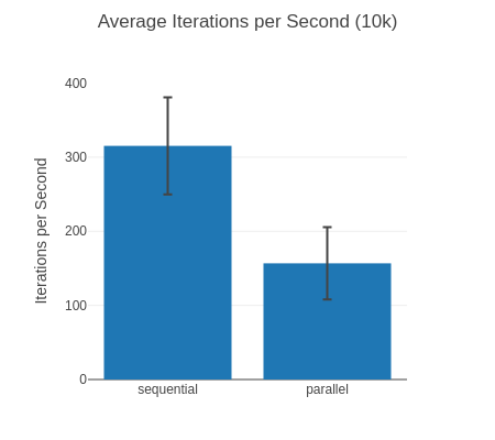
##### With input 10k #####
Name ips average deviation median 99th %
sequential 315.29 3.17 ms ±20.76% 2.96 ms 5.44 ms
parallel 156.77 6.38 ms ±31.08% 6.11 ms 10.75 ms
Comparison:
sequential 315.29
parallel 156.77 - 2.01x slower +3.21 ms
Extended statistics:
Name minimum maximum sample size mode
sequential 2.61 ms 7.84 ms 18.91 K 2.73 ms, 3.01 ms
parallel 3.14 ms 11.99 ms 9.40 K4.80 ms, 4.87 ms, 8.93 ms
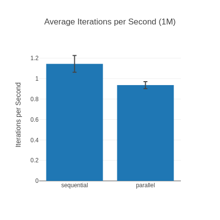
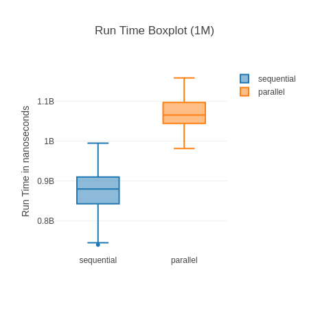
##### With input 1M #####
Name ips average deviation median 99th %
sequential 1.14 0.87 s ±7.16% 0.88 s 0.99 s
parallel 0.94 1.07 s ±3.65% 1.07 s 1.16 s
Comparison:
sequential 1.14
parallel 0.94 - 1.22x slower +0.194 s
Extended statistics:
Name minimum maximum sample size mode
sequential 0.74 s 0.99 s 69 None
parallel 0.98 s 1.16 s 57 None
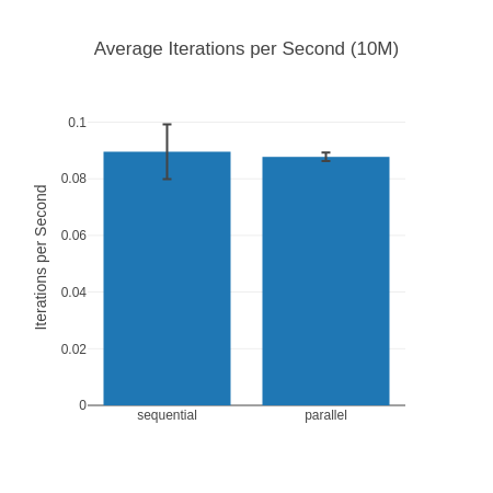
##### With input 10M #####
Name ips average deviation median 99th %
sequential 0.0896 11.17 s ±10.79% 11.21 s 12.93 s
parallel 0.0877 11.40 s ±1.70% 11.37 s 11.66 s
Comparison:
sequential 0.0896
parallel 0.0877 - 1.02x slower +0.23 s
Extended statistics:
Name minimum maximum sample size mode
sequential 9.22 s 12.93 s 6 None
parallel 11.16 s 11.66 s 6 None
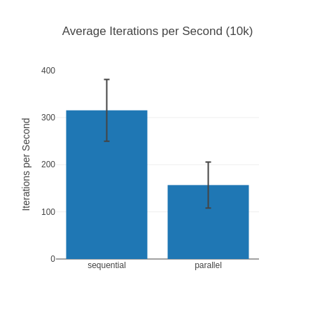
10k input, iterations per second (higher is better)
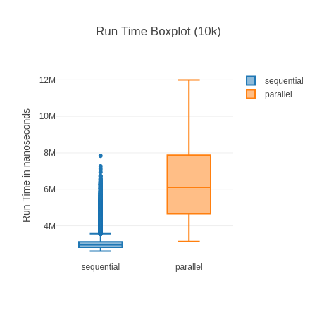
Boxplot for 10k, measured run time (lower is better). Sort of interesting how many “outliers” (blue dots) there are for sequential though.
1M input, iterations per second (higher is better)
Boxplot for 1M, measured run time (lower is better).
10M input, iterations per second (higher is better). Important to know, they take so long here the sample size is only 6 for each.
And just as we all expected the parallel… no wait a second the sequential version is faster for all of them? How could that be? This was easily parallelizable work, split into 3 work packages with many more cores available to do the work. Why is the parallel execution slower?
What happened here?
There’s no weird trick to this: It ran on a system with 12 physical cores that was idling save for the benchmark. Starting processes is extremely fast and lightweight, so that’s also not it. By most accounts, parallel processing should win out.
What is the problem then?
The problem here are the huge lists the tasks need to operate on and the return values that need to get back to the main process. The BEAM works on a “share nothing” architecture, this means in order to process theses lists in parallel we have to copy the lists over entirely to the process (Tasks are backed by processes). And once they’re done, we need to copy over the result as well. Copying, esp. big data structures, is both CPU intensive and memory intensive. In this case the additional copying work we do outweighs the gains we get by processing the data in parallel. You can also see that this effect seems to be diminishing the bigger the lists get – so it seems like the parallelization is catching up there.
The full copy may sound strange – after all we’re dealing with immutable data structures which should be safe to share. Well, once processes share data garbage collection becomes a whole other world of complex, or in the words of the OTP team in “A few notes on message passing” (emphasis mine):
Sending a message is straightforward: we try to find the process associated with the process identifier, and if one exists we insert the message into its signal queue.
Messages are always copied before being inserted into the queue. As wasteful as this may sound it greatly reduces garbage collection (GC) latency as the GC never has to look beyond a single process. Non-copying implementations have been tried in the past, but they turned out to be a bad fit as low latency is more important than sheer throughput for the kind of soft-realtime systems that Erlang is designed to build.
In case you’re interested in other factors for this particular benchmark: I chose the 3 functions semi-randomly looking for functions that traverse the full list at least once doing some non trivial work. If you do heavier work on the lists the parallel solution will fare better. We can also not completely discount that CPU boosting (where single core performance may increase if the other cores are idle) is shifting benchmark a bit in favor of sequential but overall it should be solid enough for demonstration purposes. Due to the low sample size for the 10M list, parallel execution may sometimes come out ahead, but usually doesn’t (and I didn’t want the benchmark take even longer).
The Sneakyness
Now, the problem here is a bit more sneaky – as we’re not explicitly sending messages. Our code looks like this: Task.async(fn -> Enum.uniq(big_list) end) – there is no send or GenServer.call here! However, that function still needs to make its way to the process for execution. As the closure of the function automatically captures referenced variables – all that data ends up being copied over as well! (Technically speaking Task.async does a send under the hood, but spawn/1 also behaves like this.)
This is what caught me off-guard with this – I knew messages were copied, but somehow Task.async was so magical I didn’t think about it sending messages or needing to copy its data to a process. Let’s call it a blind spot and broken mental model I’ve had for way too long. Hence, this blog post is for you dear reader – may you avoid the mistake I made!
Let’s also be clear here that normally this isn’t a problem and the benefits we get from this behavior are worth it. When a process terminates we can just free all its memory. It’s also not super common to shift so much data to a process to do comparatively lightweight work. The problem here is a bit, how easy it is for this problem to sneak up on you when using these high level abstractions like Task.async/1.
Real library, real problems
Yup. While I feel some shame about it, I’ve always been an advocate for sharing mistakes you made to spread some of the best leanings. This isn’t a purely theoretical thing I ran into – it stems from real problems I encountered. As you may know I’m the author of benchee – the best benchmarking library ™ 😉 . Benchee’s design, in a nut shell, revolves around a big data structure – the suite – data is enriched throughout the process of benchmarking. You may get a better idea by looking at the breakdown of the steps. This has worked great for us.
However, some of the data in that suite may reference large chunks of data if the benchmark operates on large data. Each Scenario references its given input as well as its benchmarking function. Given what we just learned both of these may be huge. More than that, the Configuration also holds all the configured inputs and is part of the suite as well.
Now, when benchee tries to compute your statistics in parallel it happily creates a new process for each scenario (which may be 20+) copying over the benchmarking function and input although it really doesn’t need them.
Even worse formatters are run in parallel handing over the entire suite – including all scenarios (function and input) as well as all the inputs again as part of the Configuration – none of which a formatter should need. 😱
To be clear, you will only encounter this problem if you deal with huge sets of data and if you do it’s “just” more memory and time used. However, for a library about measuring things and making them fast this is no good.
The remedy
Thankfully, there are multiple possible remedies for this problem:
Limiting the data you send to the absolute necessary minimum, instead of just sending the whole struct. For example, don’t send an entire Suite struct if all you need is a couple of fields.
If only the process needs the data, it may fetch the data itself instead. I.e. instead of putting the result of a giant query into the process, the process could be the one doing the query if it’s the only one that needs the data.
There are some data structures that are shared between processes and hence don’t need copying, such as ets and persistent_term.
As teased above, the most common and easiest solution is just to pass along the data you need, if you ended up accidentally sending along more than you wanted to. You can see one step of it in this pull request or this one.
The results are quite astounding, for a benchmark I’m working on (blog post coming soon ™) this change got it from practically being unable to run the benchmark due to memory constraints (on a 32GB RAM system) to easily running the benchmark – maximum resident size set size got almost halfed.
The magnitude of this can also be shown perhaps by the size of the files I saved for this benchmark. Saving is actually implemented as a formatter, and so automatically benefits from these changes – the file size for this benchmark went down from ~200MB per file to 1MB aka a reduction to 0.5% in size. You can read more about how it improved in the benchee 1.3.0 release notes.
Naturally this change will also make its way to you all as benchee 1.3.0 soon (edit: out now!).
Also when pursuing to fix this be mindful that you need to completely remove the variable from the closure. You can’t just go: Task.async(fn -> magic(suite.configuration) end) – the entire suite will still be sent along.
iex(1)> list = Enum.to_list(1..100_000)
iex(2)> # do not benchmark in iex, this is purely done to get a suite with some data
iex(3)> suite = Benchee.run(%{map: fn -> Enum.map(list, fn i -> i * i end) end })
iex(4)> :erts_debug.size(suite)
200642
iex(5)> :erts_debug.size(fn -> suite end)
200675
iex(6)> :erts_debug.size(fn -> suite.configuration end)
200841
iex(7)> :erts_debug.size(fn -> suite.configuration.time end)
201007
iex(8)> configuration = suite.configuration
iex(9)> :erts_debug.size(fn -> configuration.time end)
295
iex(10)> time = configuration.time
iex(11)> :erts_debug.size(fn -> time end)
54
Helping others avoid making the same mistake
All of that discovery, and partially shame, left me with the question: How can I help others avoid making the same mistake? Well, one part of it is right here – publish a blog post. However, that’s one point.
Also don’t forget: processes are still awesome and lightweight– you should use them! This is just a cautionary tale of how things might go wrong if you’re dealing with big chunks of data and that the work you’re doing on that data may not be extensive enough to warrant a full copy. Or that you’re accidentally sending along too much data unaware of the consequences. There are many more use cases for processes and tasks that are absolutely great, appropriate and will save you a ton of time.
What does this leave us with? As usual: don’t assume, always benchmark!
Also, be careful about the data you’re sending around and if you really need it! 💚
There is a known issue affecting elixir versions from 1.14.0 to 1.16.0-rc.0: Optimizations (SSA and bool passes, see the original change) had been disabled affecting the performance of functions defined directly in the top level (i.e. outside of any module). The issue was fixed by re-enabling the optimization in 1.16.0-rc.1 (commit with the fix). The issue is best show-cased by the following benchmark where we’d expect ~equal results:
list = Enum.to_list(1..10_000)

defmodule Compiled do
  def comprehension(list) do
    for x <- list, rem(x, 2) == 1, do: x + 1
  end
end

Benchee.run(%{
  "module (optimized)" => fn -> Compiled.comprehension(list) end,
  "top_level (non-optimized)" => fn -> for x <- list, rem(x, 2) == 1, do: x + 1 end
})
The benchmark yields roughly these results on an affected elixir version, which is a stark contrast:
Comparison:
module (optimized)              18.24 K
top_level (non-optimized)       11.91 K - 1.53x slower +29.14 μs
So, how do you fix it/make sure a benchmark you ran is not affected? All of these work:
benchmark on an unaffected/fixed version of elixir (<= 1.13.4 or >= 1.16.0-rc.1)
put the code you want to benchmark into a module (just like it is done in Compiled in the example above)
you can also invoke Benchee from within a module, such as:
defmodule Compiled do
  def comprehension(list) do
    for x <- list, rem(x, 2) == 1, do: x + 1
  end
end

defmodule MyBenchmark do
  def run do
    list = Enum.to_list(1..10_000)

    Benchee.run(%{
      "module (optimized)" => fn -> Compiled.comprehension(list) end,
      "top_level (non-optimized)" => fn -> for x <- list, rem(x, 2) == 1, do: x + 1 end
    })
  end
end

MyBenchmark.run()
Also note that even if all your examples are top level functions you should still follow these tips (on affected elixir versions), as the missing optimization might affect them differently. Further note, that even though your examples use top level functions they may not be affected, as the specific disabled optimization may not impact them. Better safe than sorry though 🙂
The Fun with Optimizations
A natural question here is “why would anyone disable optimizations?”, which is fair. The thing with many optimizations is – they don’t come for free! They might be better in the majority of the cases, but there is often still that part where they are slower. Think of the JVM and its great JIT – it gives you a great performance after a warmup period but during warmup it’s usually slower than without a JIT (as it needs to perform the additional JIT work). If you want to read more on warmup times I have an extensive blog post covering the topic.
So, what was the goal here? As the original PR states:
Module bodies, especially in tests, tend to be long, which affects the performance of passe such as beam_ssa_opt and beam_bool. This commit disables those passes during module definition. As an example, this makes loading Elixir’s test suite 7-8% faster.
José Valim
Which naturally is a valid use case and a good performance gain. The unintended side effect here was, that it also affected “top level functions”/functions outside of any module which in 99.99% of cases doesn’t matter and can be ignored. Let me reiterate this, this should not have affected any of your applications.
The problem here is that benchee was affected – as for ease of use we usually forego the definition of modules (while it’s completely possible). And well, optimizations not being in effect when used with a benchmarking library is quite the problem 😐 😭 Hence, this blog post along with a notice in the README to raise awareness.
So, if you ran benchmarks on affected elixir versions I recommend checking the above scenario and redoing the benchmarks with the above fixes applied.
On the positive side, I’m happy how quickly we got around to the issue after it was discovered, Jean opened the issue only 4 days after it was fixed in elixir and a day after it was released as part of the 1.16.0-rc.1. So, huge shout out and thank you again!
And for even more positive news: does this now mean our tests load slower again just so benchee can function without module definitons? No! At least as best as I understand the fix, it increases the precision by disabling the compiler optimizations only in module bodies.
I’m glad that that’s all, not to say I don’t have ideas on what else to improve although I won’t promise things. It’s great that benchee just works. It’s a mature piece of software that works well. We need to move away from declaring projects that haven’t seen a release in a while as “dead”. That said, of course some occasional updates on the repo to make sure they work with the most recent versions would be nice.
In particular I’m happy that benchee already started out with warmup as simply the right thing to do(tm). So, when erlang implemented a JIT I had nothing new to do as I new benchee already supported it perfectly.
And that’s also true for all of benchee’s “sister” libraries. I took some time for some house cleaning today to fix their CIs and run them against all the newest versions and… none of them needed any meaningful adjustment that would warrant a new release. That makes me happy.
Benchee 1.1.0 has finally hit hex.pm. After, well, almost 3 years. So, in this blog post we’ll dive into:
What are the changes
Why did it take so long, with some (significant) musings on Open Source and bugs as well as my approach to it
What does Benchee 1.1.0 Bring to the table
The star of the show certainly are the two new major features: reduction measurements and profiling! Then there is also a nasty bug that was squashed. Check out the Changelog for all.
Reduction Counting
Reductions joins execution time and memory consumption as the third measure Benchee can take. This one was kicked off way back when someone asked in our #benchee channel about adding this feature. What reductions are, is hard to explain. In short, it’s not very well defined but a “unit of work”. The BEAM uses them to keep track of how long a process has run. As the Beam Book puts it as follows:
BEAM solves this by keeping track of how long a process has been running. This is done by counting reductions. The term originally comes from the mathematical term beta-reduction used in lambda calculus.
The definition of a reduction in BEAM is not very specific, but we can see it as a small piece of work, which shouldn’t take too long. Each function call is counted as a reduction. BEAM does a test upon entry to each function to check whether the process has used up all its reductions or not. If there are reductions left the function is executed otherwise the process is suspended.
This can help you, as it’s not affected by system load so you could make assumptions in your CI about performance. It’s not 1:1 but it helps. Of course, check out Benchee’s docs about it. Biggest shout out goes to Devon for implementing it.
You can simply specify reduction_time and there you go:
This file contains bidirectional Unicode text that may be interpreted or compiled differently than what appears below. To review, open the file in an editor that reveals hidden Unicode characters.
Learn more about bidirectional Unicode characters
This file contains bidirectional Unicode text that may be interpreted or compiled differently than what appears below. To review, open the file in an editor that reveals hidden Unicode characters.
Learn more about bidirectional Unicode characters
It’s worth noting that reduction counts will differ between different elixir and erlang versions – as we often noticed in our own CI setup.
Profile after benchmarking
Another feature that I’d never imagined having in Benchee, but thanks to community suggestions (and implementation!) it came to be. This one in particular was even suggested by José Valim himself – chatting with him he asked if there were plans to include something like this as his workflow would often be:
1. benchmark to see results
2. profile to find improvement opportunities
3. improve code
4. Start again at 1.
Makes perfect sense, I just never thought of it. So, you can now say profile_after: true or even specify a specific profiler + options.
This file contains bidirectional Unicode text that may be interpreted or compiled differently than what appears below. To review, open the file in an editor that reveals hidden Unicode characters.
Learn more about bidirectional Unicode characters
This file contains bidirectional Unicode text that may be interpreted or compiled differently than what appears below. To review, open the file in an editor that reveals hidden Unicode characters.
Learn more about bidirectional Unicode characters
We didn’t implement the profiling ourselves, but instead we rely on the builtin profiling tasks like this one. To make the feature fully compatible with hooks, I also had to send a small patch to elixir and so after_each hooks won’t work with profiling until it’s released. But, nobody uses hooks anyhow so, who cares? 😛
This feature made it in thanks to Pablo Costas, and his great work. I’m happy to highlight that not only did this contribution give us all a great Benchee feature, but also a friendship to boot. Oh, the wonders of Open Source. 💚
Measurement accuracy on Mac
Now to the least fun part about this release. There is a bugfix, a quite important one at that. Basically on Mac OS previous Benchee versions might report inaccurate results for very fast benchmarks (< 10 microseconds). There are many more musings in this issue, but basically we relied on the operating system clock returning times in a value that it can accurately measure in. Alas, OSX reports in nanoseconds but only has microsecond accuracy (leading to measurements being multiples of 1000). However, even the operating system clock reported nanosecond accuracy – so I even reported a bug on erlang/otp that was thankfully fixed in 22.2.
Fixing this was hard and stressful, which leads nicely into the next major section…
Why it took so long, perfectionism and open source
So, why did it take so long? I blogged earlier today about some of the things that held me back the past 1.5 years in “The Silence Between”. However, you can see that a lot of these features already landed in early 2020, so what gives?
The short answer is the bug above was hard to fix and I needed to fix it. The long answer is… well, long.
I think I could describe myself as a pragmatic perfectionist. I’m happy to implement an MVP, I constantly ask “Do we really need this?” or “Can we make this simpler and deliver it faster?”, but what I end up shipping I want to… well, almost need to be great for what we decided to ship. I don’t want to release with bugs, constant error notifications or barely anything tested. I can make lots of tradeoffs, as long as I decide on them like: Ok we’ll duplicate this code now, as we have no idea what a good abstraction might be and we don’t wanna lock ourselves in. But something misbehaving that I thought was sublime? Oh, the pain.
Why am I highlighting this? Well, Benchee reporting wrong resultsis frightening to me. Benchee has one core promise, and that promise is to measure your functions as accurately as possible. Also, in my opinion fixing critical bugs such as this one should have the highest priority. I can’t, for myself, justify working on Benchee while not working on that bug. I know, it’s not a great attitude and I should have released the features on main and just released the bug fix later. I do. But I felt like, all energy had to be spent on fixing that bug.
And working on that bug was hard. It’s a Mac only bug and I famously do not own or want to own a Mac. My partner owns one, but when I’m doing Open Source chances are she’s at her computer as well. And then, to investigate something like this, I need a couple of hours of interrupted time with no distractions on my mind as well. I might as well not even start otherwise. It certainly didn’t help that the bug randomly disappeared, when trying to look at it.
The problem that I did not have a Mac to fix this was finally solved when I started a new job, but then first the stress was too high and then my arms were injured (as mentioned in the other blog post). My arms finally got better and I had a good 4h+ to set aside to fix this bug. It can be kind of hard, to get that dedicated time but it’s absolutely needed for an intricate bug such as this one.
So, that’s the major reason it took so long. I mean, it involved finding a bug in Erlang itself. And, me working around that bug which is some code that well… was almost harder to write than the actual fix.
I would be amiss not to mention something else: It’s perfectly fine for Open Source project not to update! Sometimes, they are just done. Or the maintainers have more important things to do. I certainly consider Benchee “done” since 1.0 as it has all features I really wanted it to have. You see, reduction counting and profiler after are great features, but they are hardly essential.
Still, Benchee having a rather important bug for so long really made me feel guilty and bad. Even worse, because I didn’t fix the bug those great contributions from Devon and Pablo were never released. That’s another thing, that’s very important to me: Whoever takes the time to contribute should have a great experience and their contribution should be valued. The ultimate show of appreciation is releasing the feature they worked on is getting it released into people’s hands.
At times those negative feelings (“Oh no there is a bug” & “Oh no these great features lie around unreleased”) paradoxically lead me to stay away from Benchee even more since I felt bad about this state. Yes, it was only on mac and only affected benchmarks where individual function invocations took less than 10 microseconds. But still, that’s the perfectionist in me. This should be fixed within weeks, not 2.5 years. Most certainly, ready to ship features shouldn’t just chill on main for years. Release early, release often.
Anyhow, thanks for reading my musings on Open Source, responsibility, pragmatism and perfectionism. The bug is fixed now, the features are released and I’m happy. Who knows what’s next for Benchee.
Ever wanted to implement something board game like in Elixir? Chess? Go? Islands? Well, then you’re gonna need a board!
But what data structure would be the most efficient one to use in Elixir? Conventional wisdom for a lot of programming languages is to use some sort of array. However, most programming languages with immutable data structures don’t have a “real” array data structure (we’ll talk about erlangs array later, it’s not really like the arrays in non functional languages) . Elixir is one of those languages.
For this benchmark I didn’t have a very specific board game in mind so I settled for a board size of 9×9 . It’s a bit bigger than a normal chess board (8×8), it’s exactly the size of the smallest “normal” Go-board and it’s one smaller than the board used in Islands implemented in Functional Web Development with Elixir, OTP and Phoenix, so it seemed like a good compromise. Different sizes are likely to sport different performance characteristics.
Without a concrete usage scenario in mind I settled on a couple of different benchmarks:
getting a value at the coordinates (0,0), (4, 4) and (8,8). This is a fairly nano/micro benchmark for data access and provides a good balance of values at the beginning/middle/end when thinking in list terms.
setting a value at the coordinates (0,0), (4, 4) and (8,8).
a still nano/micro benchmark that combines the two previous benchmarks by getting and setting all three mentioned values. I call this “mixed bag”.
Why stop at the previous one? The last benchmark just sets and gets every possible coordinate once (first it sets (0,0) then gets it, then it sets (0, 1), then gets it and so forth). This also simulates the board filling which can be important for some data structures. Completely filling a board is unrealistic for most board games however, as most games finish before this stage. This one is called “getting and setting full board”.
Something that is notably not benchmarked is the creation of boards. For (almost) all of the board implementations it could resolve to a constant value which should be similar in the time it takes to create. I wasn’t overly interested in that property and didn’t want to make the code less readable by inlining the constant after creation when I didn’t need to.
Also noteworthy is that these benchmark mostly treat reading and writing equally while in my experience most AIs/bots are much more read-heavy than write-heavy.
Take all these caveats of the benchmark design into consideration when looking at the results and if in doubt of course best write your own benchmark taking into account the concrete usage patterns of your domain.
Without further ado then let’s look at the different implementations I have benchmarked so far:
This file contains bidirectional Unicode text that may be interpreted or compiled differently than what appears below. To review, open the file in an editor that reveals hidden Unicode characters. Learn more about bidirectional Unicode characters
All boards are built so that accessing a previously unset field will return nil. No assumptions about the data stored in the board have been made, which rules out String as an implementation type. In the benchmarks atoms are used as values.
In the descriptions of the data types below (x, y) is used to mark where what value is stored.
List2D: A 2 dimensional list representing rows and columns: [[(0, 0), (0, 1), (0, 2), ...], [(1, 0), (1, 1), ..], ..., [..., (8, 8)]]
List1D: Using the knowledge of a constant board size you can encode it into a one-dimensional list resolving the index as dimension * x + y: [(0, 0), (0, 1), (0, 2), ..., (1, 0), (1, 1), ..., (8, 8)]
Tuple2D: Basically like List2D but with tuples instead of lists: {{(0, 0), (0, 1), (0, 2), ...}, {(1, 0), (1, 1), ..}, ..., {..., (8, 8)}}
Tuple1D: Basically like List1D but with a tuple instead of a list: {(0, 0), (0, 1), (0, 2), ..., (1, 0), (1, 1),... (8, 8)}
Array1D: see above for the data structure in general, otherwise conceptually like Tuple1D.
MapTuple: A map that takes the tuple of the coordinates {x, y} as the key with the value being whatever is on the board: %{{0, 0} => (0, 0), {0, 1} => (0, 1), ..., {8, 8} => (8, 8)}. It’s a bit unfair compared to others shown so far as it can start with an empty map which of course is a much smaller data structure that is not only smaller but usually faster to retrieve values from. As the benchmarks start with an empty board that’s a massive advantage, so I also included a full map in the benchmark, see next/
MapTupleFull: Basically the same as above but initialized to already hold all key value pairs initialized as nil. Serves not only the purpose to see how this performs but also to see how MapTuple performs once it has “filled up”.
MapTupleHalfFull: Only looking at complete full performance and empty performance didn’t seem good either, so I added another one initialized from 0 to 4 on all columns (a bit more than a board half, totalling 45 key/value pairs).
MapTupleQuarterFull: Another one of these, this time with 27 key/value pairs. Why? Because there is an interesting performance characteristic, read on to find out 🙂
Map2D: Akin to List2D etc. a map of maps: %{0 => %{0 => (0, 0), 1 => (0, 1), ...}, 1 => %{0 => (1, 0), ...}, ..., 8 => %{..., 8 => (8, 8)}}
ETSSet: erlang ETS storage with table type set. Storage layout wise it’s basically the same as MapTuple, with a tuple of coordinates pointing at the stored value.
ETSOrderedSet: Same as above but with table type ordered_set.
ProcessDictionary: On a special request for Michał 😉 This is probably not a great default variant as you’re practically creating (process-) global state which means you can’t have two boards within the same process without causing mayham. Also might accidentally conflict with other code using the process dictionary. Still might be worth considering if you want to always run a board in its own process.
It’s significant to point out that all mentioned data types except for ETS and the process dictionary are immutable. This means that especially for those in the benchmark a new board is created in a before_each hook (does not count towards measured time) to avoid “contamination”.
Another notable exception (save for String for the aforementioned constraints) is Record. Records are internally represented as tuples but give you the key/value access of maps, however in elixir it is more common to use Structs (which are backed by maps). As both maps and tuples are already present in the benchmark including these likely wouldn’t lead to new insights.
System Setup
Operating System
Linux
CPU Information
Intel(R) Core(TM) i7-4790 CPU @ 3.60GHz
Number of Available Cores
8
Available Memory
15.61 GB
Elixir Version
1.8.2
Erlang Version
22.0
Benchmarking Results
Benchmarks of course were run with benchee and the benchmarking script is here (nothing too fancy).
You can check them out in the repo as markdown (thanks to benchee_markdown) or HTML reports (benchee_html). Careful though if you’re on mobile some of the HTML reports contain the raw measurements and hence go up to 9MB in size and can take a while to load also due to the JS drawing graphs!
getting and setting full board iterations per second (higher is better)
It’s a tight race at the top when it comes to run time! Tupl1D, Tuple2D and MapTuple are all within striking range of each other and then there’s a sharp fall off.
Also there is a fair bit of variance involved as shown by the black “whiskers” (this is usual for benchmarks that finish in nanoseconds or microseconds because of garbage collection, interference etc.). Which one of these is best? To get a better picture let’s look at the whole table of results:
Name
IPS
Average
Deviation
Median
Mode
Minimum
Maximum
Tuple1D
133.95 K
7.47 μs
±23.29%
6.93 μs
6.88 μs
6.72 μs
492.37 μs
Tuple2D
132.16 K
7.57 μs
±29.17%
7.21 μs
7.16 μs
7.03 μs
683.60 μs
MapTuple
126.54 K
7.90 μs
±25.69%
7.59 μs
7.56 μs
7.43 μs
537.56 μs
ProcessDictionary
64.68 K
15.46 μs
±14.61%
15.12 μs
15.05 μs
14.89 μs
382.73 μs
ETSSet
60.35 K
16.57 μs
±9.17%
16.04 μs
15.95 μs
15.79 μs
161.51 μs
Array2D
56.76 K
17.62 μs
±17.45%
17.15 μs
17.04 μs
16.54 μs
743.46 μs
MapTupleFull
55.44 K
18.04 μs
±11.00%
16.92 μs
16.59 μs
16.43 μs
141.19 μs
MapTupleHalfFull
53.70 K
18.62 μs
±8.36%
17.96 μs
17.87 μs
17.67 μs
160.86 μs
Array1D
50.74 K
19.71 μs
±10.60%
19.29 μs
18.99 μs
18.81 μs
469.97 μs
ETSOrderedSet
39.53 K
25.30 μs
±10.51%
24.82 μs
24.57 μs
24.34 μs
390.32 μs
Map2D
36.24 K
27.59 μs
±8.32%
27.71 μs
25.90 μs
25.12 μs
179.98 μs
List2D
29.65 K
33.73 μs
±4.12%
33.31 μs
33.04 μs
31.66 μs
218.55 μs
MapTupleQuarterFull
28.23 K
35.42 μs
±3.86%
34.96 μs
34.61 μs
34.39 μs
189.68 μs
List1D
15.41 K
64.90 μs
±2.84%
64.91 μs
64.14 μs
62.41 μs
175.26 μs
Median, and Mode are good values to look at when unsure what is usually fastest. These values are the “middle value” and the most common respectively, as such they are much less likely to be impacted by outliers (garbage collection and such). These seem to reinforce that Tuple1D is really the fastest, if by a negligible margin.
MapTuple is very fast, but its sibling MapTupleFull, that already starts “full”, is more than 2 times slower. Whether this is significant for you depends if you start with a truly empty board (Go starts with an empty board, chess doesn’t for instance).
Somewhat expectedly List1D does worst as getting values towards to the end of the list it has to traverse the entire list which is incredibly slow.
As an aside, it’s easy to see in the box plot that the high deviation is mainly caused by some very big outliers:
Boxplot of getting and setting full board – dots are outliers
The dots denote outliers and they are so big (but few) that the rest of the chart is practically unreadable as all that remains from the actual box is practically a thick line.
What about memory consumption?
getting and setting full board memory usage (lower is better)
Here we can see the immediate drawback of Tuple1D – it’s memory consumption is many times worse than that of the others. My (educated) guess is that it’s because it has to replace/copy/update the whole tuple with it’s 9*9 = 81 values for every update operation. Tuple2D is much more economical here, as it only needs to to update the tuple holding the columns and the one holding the specific column we’re updating (2 * 9 = 18) to the best of my understanding.
Big Tuples like this are relatively uncommon in “the real world” in my experience though as their fixed size nature makes them inapplicable for a lot of cases. Luckily, our case isn’t one of them.
MapTuple does amazingly well overall as it’s probably the structure quite some people would have intuitively reached for for good constant memory access speed. It’s memory consumption is also impressively low.
ProcessDictionary is very memory efficient and also constantly in the top 4 when it comes to run time. However, at least run time wise there’s quite the margin ~15 μs to ~7 μs which doesn’t seem to make the risks worth it overall.
Other Observations
Let’s take a look at some other things that seem note worthy:
ETS isn’t the winner
This surprised me a bit (however I haven’t used ETS much). ETS was always tagged as the go to option for performance in my mind. Looking at the docs and use cases I know it makes sense though – we’re likely to see benefits for much larger data sets as ours is relatively small:
These (ETS) provide the ability to store very large quantities of data in an Erlang runtime system, and to have constant access time to the data.
Let’s have a look at some of the time it takes to retrieve a value – usually a much more common operation than writing:
get(0,0)
Name
IPS
Average
Deviation
Median
Mode
Minimum
Maximum
Tuple1D
44.12 M
22.66 ns
±842.77%
20 ns
20 ns
9 ns
35101 ns
Tuple2D
42.46 M
23.55 ns
±846.67%
20 ns
19 ns
7 ns
36475 ns
Array1D
30.38 M
32.92 ns
±84.61%
32 ns
32 ns
20 ns
8945 ns
MapTuple
29.09 M
34.38 ns
±111.15%
32 ns
31 ns
19 ns
10100 ns
MapTupleQuarterFull
18.86 M
53.03 ns
±37.27%
50 ns
49 ns
38 ns
2579 ns
Array2D
18.62 M
53.70 ns
±67.02%
50 ns
49 ns
34 ns
10278 ns
List1D
18.26 M
54.75 ns
±56.06%
53 ns
52 ns
42 ns
8358 ns
ProcessDictionary
17.19 M
58.18 ns
±1393.09%
52 ns
51 ns
39 ns
403837 ns
Map2D
15.79 M
63.34 ns
±25.86%
60 ns
54 ns
41 ns
388 ns
MapTupleHalfFull
10.54 M
94.87 ns
±27.72%
91 ns
89 ns
76 ns
2088 ns
MapTupleFull
10.29 M
97.16 ns
±18.01%
93 ns
89 ns
70 ns
448 ns
ETSSet
9.74 M
102.63 ns
±26.57%
100 ns
99 ns
78 ns
2629 ns
List2D
9.04 M
110.57 ns
±69.64%
105 ns
109 ns
82 ns
4597 ns
ETSOrderedSet
6.47 M
154.65 ns
±19.27%
152 ns
149 ns
118 ns
1159 ns
get(8, 8)
Name
IPS
Average
Deviation
Median
Mode
Minimum
Maximum
Tuple2D
42.47 M
23.55 ns
±788.60%
21 ns
20 ns
7 ns
33885 ns
Tuple1D
40.98 M
24.40 ns
±725.07%
22 ns
21 ns
10 ns
34998 ns
Array1D
29.67 M
33.70 ns
±161.51%
33 ns
32 ns
21 ns
18301 ns
MapTuple
28.54 M
35.03 ns
±986.95%
32 ns
32 ns
20 ns
230336 ns
ProcessDictionary
19.71 M
50.73 ns
±1279.45%
47 ns
47 ns
34 ns
377279 ns
Array2D
17.88 M
55.92 ns
±85.10%
52 ns
51 ns
35 ns
13720 ns
Map2D
13.28 M
75.31 ns
±32.34%
73 ns
65 ns
56 ns
2259 ns
MapTupleHalfFull
12.12 M
82.53 ns
±31.49%
80 ns
80 ns
60 ns
1959 ns
ETSSet
9.90 M
101.05 ns
±16.04%
99 ns
95 ns
78 ns
701 ns
MapTupleFull
9.85 M
101.53 ns
±19.29%
99 ns
90 ns
70 ns
487 ns
ETSOrderedSet
5.59 M
178.80 ns
±41.70%
169 ns
170 ns
135 ns
4970 ns
MapTupleQuarterFull
4.09 M
244.65 ns
±16.85%
242 ns
240 ns
226 ns
9192 ns
List2D
3.76 M
265.82 ns
±35.71%
251 ns
250 ns
231 ns
9085 ns
List1D
1.38 M
724.35 ns
±10.88%
715 ns
710 ns
699 ns
9676 ns
The top 3 remain relatively unchanged. What is very illustrative to look at is List1D and List2D though. For get(0, 0) List1D vastly outperforms its 2D sibling even being closest to the top group. That is easy to explain because it basically translates to looking at the first element of the list which is very fast for a linked list. However, looking at the last element is very slow and this is what get(8, 8) translates to. All elements have to be traversed until the end is reached. As such the whole thing is almost 16 times slower for List1D. List2D is still very slow but through it’s 2-dimenstional structure it only needs to look at 18 elements instead of 81.
MapTuple vs. MapTupleQuarterFull vs. MapTupleHalfFull vs. MapTupleFull
In most scenarios, including the biggest scenario, MapTupleQuarterFull performs worse than MapTuple (expected), MapTupleHalfFull (unexpected) and MapTupleFull (unexpected). I had expected its performance to be worse than MapTuple but better than MapTupleFull and MapTupleHalfFull. Why is that?
I had no idea but Johanna had one: it might have to do with the “magic” limit at which a map “really” becomes a map and not just a list that is linearly searched. That limit is defined as 32 entries in the erlang source code (link also provided by Johanna). Our quarter full implementation is below that limit (27 entries) and hence often performance characteristics more akin to List1D (see good get(0, 0) performance but bad get(8, 8) performance) than its “real” map cousins.
To the best of my understanding this “switch the implementation at size 32” is a performance optimization. With such a small data set a linear search often performs better than the overhead introduced by hashing, looking up etc. You can also see that the trade-off pays off as in the big benchmark where the whole board is filled incrementally MapTuple (which is initially empty and grows) still provides top performance.
What I still don’t fully understand is that sometimes MapTupleFull seems to still outperform MapTupleHalfFull – but only by a very negligible margin (most notably in the “big” getting and setting full board benchmark). The difference however is so small that it doesn’t warrant further investigation I believe, unless you have an idea of course.
Performance difference of Array vs. Tuple
In the introduction I said arrays are backed by tuples – how come their performance is way worse then? Well, let’s have a look at what an array actually looks like:
It cleverly doesn’t even initialize all the fields but uses some kind of length encoding saying “the value is the default value of nil for the next 100 fields” but also saving its set size limit of 81 (fun fact: these arrays can be configured to also dynamically grow!).
Once we set a value (at index 13) the representation changes showing still some length encoding “there is nothing here for the first 10 entries” but then the indexes 10..19 are expanded as a whole tuple that’s holding our value. So, to the best of my understanding arrays work by adding “stretches” of tuples the size of 10 as they need to.
However, our custom tuple implementations are perfectly sized to begin with and not too huge. Moreover, their whole size being set at compile-time probably enables some optimizations (or so I believe). Hence the tuple implementations outperform them while arrays don’t do too shabby (especially with read access) as compared to other implementations.
Conclusion
Tuples can be very good for the use case of known at compile time sized collections that need fast access and a simple flat map performs amazingly well. All that least for the relatively small board size (9×9 = 81 fields) benchmarked against here. There is a big caveat for the map though – it is so fast if we can start with an empty map and grow it in size as new pieces are set. The completely initialized map (MapTupleFull) performs way worse, tuples are the clear winners then.
Missing a data structure? Please do a PR! There’s a behaviour to implement and then just to lists to add your module name to – more details.
Update 1 (2019-06-17): Fixed MapTupleHalfFull. Before the update it was actually just quarter full 😅 which has wildly different performance characteristics for reasons now described along with the MapTupleQuarterFull implementation. Thanks goes to Johanna for pointing that out. Also the process registry has been added as another possible implementation on a suggestion from Michał 😉 . Also added a run time box plot to show outliers clearer and visually.
All the way back in June 2016 I wrote a well received blog post about tail call optimization in Elixir and Erlang. It was probably the first time I really showed off my benchmarking library benchee, it was just a couple of days after the 0.2.0 release of benchee after all.
Tools should get better over time, allow you to do things easier, promote good practices or enable you to do completely new things. So how has benchee done? Here I want to take a look back and show how we’ve improved things.
What’s better now?
In the old benchmark I had to:
manually collect Opearting System, CPU as well as Elixir and Erlang version data
manually create graphs in Libreoffice from the CSV output
be reminded that performance might vary for multiple inputs
crudely measure memory consumption in one run through on the command line
The new benchee:
collects and shows system information
produces extensive HTML reports with all kinds of graphs I couldn’t even produce before
has an inputs feature encouraging me to benchmark with multiple different inputs
is capable of doing memory measurements showing me what consumers more or less memory
I think that these are all great steps forward of which I’m really proud.
This file contains bidirectional Unicode text that may be interpreted or compiled differently than what appears below. To review, open the file in an editor that reveals hidden Unicode characters. Learn more about bidirectional Unicode characters
This file contains bidirectional Unicode text that may be interpreted or compiled differently than what appears below. To review, open the file in an editor that reveals hidden Unicode characters. Learn more about bidirectional Unicode characters
We can easily see that the tail recursive functions seem to always consume more memory. Also that our tail recursive implementation with the switched argument order is mostly faster than its sibling (always when we look at the median which is worthwhile if we want to limit the impact of outliers).
Such an (informative) wall of text! How do we spice that up a bit? How about the HTML report generated from this? It contains about the same data but is enhanced with some nice graphs for comparisons sake:
It doesn’t stop there though, some of my favourite graphs are the once looking at individual scenarios:
This Histogram shows us the distribution of the values pretty handily. We can easily see that most samples are in a 100Million – 150 Million Nanoseconds range (100-150 Milliseconds in more digestible units, scaling values in the graphs is somewhere on the road map ;))
Here we can just see the raw run times in order as they were recorded. This is helpful to potentially spot patterns like gradually increasing/decreasing run times or sudden spikes.
Something seems odd?
Speaking about spotting, have you noticed anything in those graphs? Almost all of them show that some big outliers might be around screwing with our results. The basic comparison shows pretty big standard deviation, the box plot one straight up shows outliers (little dots), the histogram show that for a long time there’s nothing and then there’s a measurement that’s much higher and in the raw run times we also see one enormous spike.
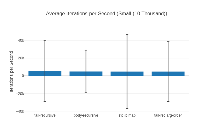
All of this is even more prevalent when we look at the graphs for the small input (10 000 elements):
Why could this be? Well, my favourite suspect in this case is garbage collection. It can take quite a while and as such is a candidate for huge outliers – the more so the faster the benchmarks are.
So let’s try to take garbage collection out of the equation. This is somewhat controversial and we can’t take it out 100%, but we can significantly limit its impact through benchee’s hooks feature. Basically through adding after_each: fn _ -> :erlang.garbage_collect() end to our configuration we tell benchee to run garbage collection after every measurement to minimize the chance that it will trigger during a measurement and hence affect results.
You can have a look at it in this HTML report. We can immediately see in the results and graphs that standard deviation got a lot smaller and we have way fewer outliers now for our smaller input sizes:
Note however that our sample size also went down significantly (from over 20 000 to… 30) so increasing benchmarking time might be worth while to get more samples again.
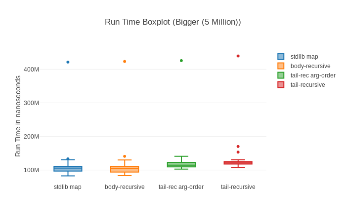
How does it look like for our big 5 Million input though?
Not much of an improvement… Actually slightly worse. Strange. We can find the likely answer in the raw run time graphs of all of our contenders:
The first sample is always the slowest (while running with GC it seemed to be the third run). My theory is that for the larger amount of data the BEAM needs to repeatedly grow the memory of the process we are benchmarking. This seems strange though, as that should have already happened during warmup (benchee uses one process for each scenario which includes warmup and run time). It might be something different, but it very likely is a one time cost.
To GC or not to GC
Is a good question. Especially for very micro benchmarks it can help stabilize/sanitize the measured times. Due to the high standard deviation/outliers whoever is fastest can change quite a lot on repeated runs.
However, Garbage Collection happens in a real world scenario and the amount of “garbage” you produce can often be directly linked to your run time – taking the cleaning time out of equation can yield results that are not necessarily applicable to the real world. You could also significantly increase the run time to level the playing field so that by the law of big numbers we come closer to the true average – spikes from garbage collection or not.
Wrapping up
Anyhow, this was just a little detour to show how some of these graphs can help us drill down and find out why our measurements are as they are and find likely causes.
The improvements in benchee mean the promotion of better practices and much less manual work. In essence I could just link the HTML report and then just discuss the topic at hand (well save the benchmarking code, that’s not in there… yet 😉 ) which is great for publishing benchmarks. Speaking about discussions, I omitted the discussions around tail recursive calls etc. with comments from José Valim and Robert Virding. Feel free to still read the old blog post for that – it’s not that old after all.
The first benchee release was almost 3 years ago – it started a mission to improve benchmarking tooling in the elixir eco system. And now we’re not at the goal – after all it’s never done and we’re not short of ideas of what to do.
What’s in a 1.0?
Also called “Why did you take so long to call it 1.0?” – 1.0 for me means a good level of stability. A level where not every second new benchee version all formatters would need updates because they would break otherwise. And in recent releases we have still shuffled major data structures around A LOT (just check all the Breaking Changes (Plugins)). Benchee was mostly stable from a user perspective – but this means it’s less of a risk factor to go ahead and write your own plugins, something that benchee always encouraged/was built to empower. I don’t have any plans for 2.0 right now – all features that I know of can easily be added to the existing structure.
It also means I’m happy with the features. What benchee offers is great, we have:
nano second precise run time measurements
memory measurements
rich statistics
show information such as CPU, elixir and erlang versions about the system running the benchmarks
support for multiple inputs
hooks to support even unconventional scenarios
you can access it all via your CLI, CSV, JSON or HTML (including nice graphs!)
and actually a lot more 😉
Benchee might have started out as “I want benchmark-ips in elixir” but it has surpassed it in many ways so that I’d actually want to have benchee in Ruby but that’s another topic. However, that makes me proud of what we accomplished.
With that amount of polish I can also easily sit back and not work on benchee for some time because I know it’s good – it is “done” in the sense that it can do everything I wanted it to do when I started the project (and even more!).
As for what is actually in it mostly removing deprecations. You can check out the Changelog.
What’s 0.99?
I found it nice how rspec did their 2.99 –> 3.0 switch – get it to run on 2.99 without deprecation warnings and then you can safely use 3.0. That was a great user experience. Ember.js handles their major versions similarly. Now, benchee is nowhere near as complex as those 2 but we thought providing that nicety would still be great.
Features
As mentioned before 0.99/1.0 don’t actually include many features – the previous 0.14.0 release from about a month ago was very feature packed. These releases are a lot about polish. Redoing the documenation, updating names, fixing typespecs, being more careful about what is and isn’t exposed in the public interface.
A small but important feature made it in though – displaying the absolute difference between measurements:
Comparison:
flat_map           2.34 K
map.flatten        1.22 K - 1.92x slower +393.09 μs
See that little+393.09 μs? It’s how much slower it was on average in absolute terms. With these comparisons people often focus too much on “OMG it’s almost 2 times as slow!!!” but this number helps put it into context: It’s not even half a millisecond. If you only do this once in a web request the difference likely doesn’t matter. It’s a calculation I always did in my head, I’m happy to make it easily accessible for everyone.
Along with this patch those values were added to our Statistics struct – including the “x-times slower” values, which means formatters no longer have to implement this themselves! Hooray!
We’re an org now!
An astute observer might have seen that all my benchee repos have been moved to the github organization bencheeorg. What’s that all about? It’s mostly a tribute to benchee not being a personal project but a community project. Many people have contributed massively to benchee, most notably Devon and Eric. Without Devon we probably still wouldn’t have memory measurements and without Eric our unit scaling wouldn’t be as great as it is. Others such as Michał and OvermindDL1 have also contributed a lot through ideas, testing and help (especially with memory measurements :)). Feels wrong to keep the repositories attached to a single person.
Also, should anything happen to me (which I hope won’t happen), the others could still add people to the organization and carry on.
It also helps with another problem I’ve had: I want to extract small useful libraries from benchee: Statistics (introduced by me), System Information gathering (introduced by Devon) and unit scaling (introduced by Eric) – where do I put these repos? All under their own name space? All under my name space? Nah, I put them in the benchee organization where we share ownership – that’s where they belong.
Help with all of those is very welcome. Personally, I’m really itching to extract these libraries I mentioned – let’s see about that. Also to showcase benchee with some nice benchmarks – after all what good is a great benchmarking tool if you rarely use it?
Long time since the last benchee release, heh? Well, this one really packs a punch to compensate! It brings you a higher precision while measuring run times as well as a better way to specify formatter options. Let’s dive into the most notable changes here, the full list of changes can be found in the Changelog.
Of course, all formatters are also released in compatible versions.
Nanosecond precision measurements
Or in other words making measurements 1000 times more precise 💥
This new version gives you much more precision which matters especially if you benchmark very fast functions. It even enables you to see when the compiler might completely optimize an operation away. Let’s take a look at this in action:
This file contains bidirectional Unicode text that may be interpreted or compiled differently than what appears below. To review, open the file in an editor that reveals hidden Unicode characters.
Learn more about bidirectional Unicode characters
This file contains bidirectional Unicode text that may be interpreted or compiled differently than what appears below. To review, open the file in an editor that reveals hidden Unicode characters.
Learn more about bidirectional Unicode characters
You can see that the averages aren’t 0 ns because sometimes the measured run time is very high – garbage collection and such. That’s also why the standard deviation is huge (big difference from 0 to 23000 or so). However, if you look at the median (basically if you sort all measured values, it’s the value is in the middle) and the mode (the most common value) you see that both of them are 0. Even the accompanying memory measurements are 0. Seems like there isn’t much happening there.
So why is that? The compiler optimizes these “benchmarks” away, because they evaluate to one static value that can be determined at compile time. If you write 1 + 1 – the compiler knows you probably mean 2. Smart compilers. To avoid these, we have to trick the compiler by randomizing the values, so that they’re not clear at compile time (see the “right” integer addition).
That’s the one thing we see thanks to our more accurate measurements, the other is that we can now measure how long a map over a range with 10 elements takes (which is around 355 ns for me (I trust the mode and median more her than the average).
This file contains bidirectional Unicode text that may be interpreted or compiled differently than what appears below. To review, open the file in an editor that reveals hidden Unicode characters.
Learn more about bidirectional Unicode characters
But, in fact nanoseconds are supported! So we now have our own simple time measuring code. This is operating system dependent though, as the BEAM knows about native time units. To the best of our knowledge nanosecond precision is available on Linux and MacOS – not on Windows.
It wasn’t just enough to switch to nano second precision though. See, once you get down to nanoseconds the overhead of simply invoking an anonymous function (which benchee needs to do a lot) becomes noticeable. On my system this overhead is 78 nanoseconds. To compensate, benchee now measures the function call overhead and deducts it from the measured times. That’s how we can achieve measurements of 0ns above – all the code does is return a constant as the compiler optimized it away as the value can be determined at compile time.
A nice side effect is that the overhead heavy function repetition is practically not used anymore on Linux and macOS as no function is faster than nanoseconds. Hence, no more imprecise measurements due to function repetition to make it measurable at all (on Windows we still repeat the function call for instance 100 times and then divide the measured time by this).
Formatter Configuration
This is best shown with an example, up until now if you wanted to pass options to any of the formatters you had to do it like this:
This file contains bidirectional Unicode text that may be interpreted or compiled differently than what appears below. To review, open the file in an editor that reveals hidden Unicode characters.
Learn more about bidirectional Unicode characters
This always felt awkward to me, but it really hit hard when I watched a benchee video tutorial. There the presenter said “…here we configure the formatter to be used and then down here we configure where it should be saved to…” – why would that be in 2 different places? They could be far apart in the code. There is no immediate visible connection between Benchee.Formatters.HTML and the html: down in the formatter_options:. Makes no sense.
That API was never really well thought out, sadly. So, what can we do instead? Well of course, bring the options closer together:
This file contains bidirectional Unicode text that may be interpreted or compiled differently than what appears below. To review, open the file in an editor that reveals hidden Unicode characters.
Learn more about bidirectional Unicode characters
So, if you want to pass along options instead of just specifying the module, you specify a tuple of module and options. Easy as pie. You know exactly what formatter the options belong to.
Road to 1.0?
Honestly, 1.0 should have happened many versions ago. Right now the plan is for this to be the last release with user facing features. We’ll mingle the data structure a bit more (see the PR if interested), then put in deprecation warnings for functionality we’ll remove and call it 0.99. Then, remove deprecated functionality and call it 1.0. So, this time indeed – it should be soon ™. I have a track record of sneaking in just one more thing before 1.0 though 😅. You can track our 1.0 progress here.
Why did this take so long?
Looking at this release it’s pretty packed. It should have been 2 releases (one for every major feature described above) that should have happened much sooner.
Basically, these required updating the formatters, which isn’t particularly fun, but necessary as I want all formatters to be ready to release along a new benchee version. In addition, we put in even more work (specifically Devon in big parts) and added support for memory measurements to all the formatters.
Beyond this? Well, I think life. Life happened. I moved apartments, which is a bunch of work. Then a lot of things happened at work leading to me eventually quitting my job. Some times there’s just no time or head space for open source. I’m happy though that I’m as confident as one can be in that benchee is robust and bug free software, so that I don’t have to worry about it breaking all the time. I can already see this statement haunting me if this release features numerous weird bugs 😉
In that vain, hope you enjoy the new benchee version – happy to hear feedback, bugs or feature ideas!
And because you made it so far, you deserve an adorable bunny picture: