Revisiting “Tail Call Optimization in Elixir & Erlang” with benchee 1.0

All the way back in June 2016 I wrote a well received blog post about tail call optimization in Elixir and Erlang. It was probably the first time I really showed off my benchmarking library benchee, it was just a couple of days after the 0.2.0 release of benchee after all.

Tools should get better over time, allow you to do things easier, promote good practices or enable you to do completely new things. So how has benchee done? Here I want to take a look back and show how we’ve improved things.

What’s better now?

In the old benchmark I had to:

• manually collect Opearting System, CPU as well as Elixir and Erlang version data
• manually create graphs in Libreoffice from the CSV output
• be reminded that performance might vary for multiple inputs
• crudely measure memory consumption in one run through on the command line

The new benchee:

• collects and shows system information
• produces extensive HTML reports with all kinds of graphs I couldn’t even produce before
• has an inputs feature encouraging me to benchmark with multiple different inputs
• is capable of doing memory measurements showing me what consumers more or less memory

I think that these are all great steps forward of which I’m really proud.

Show me the new benchmark!

Here you go, careful it’s long (implementation of MyMap for reference):

	map_fun = fn i -> i + 1 end
	inputs = [
	{"Small (10 Thousand)", Enum.to_list(1..10_000)},
	{"Middle (100 Thousand)", Enum.to_list(1..100_000)},
	{"Big (1 Million)", Enum.to_list(1..1_000_000)},
	{"Bigger (5 Million)", Enum.to_list(1..5_000_000)},
	{"Giant (25 Million)", Enum.to_list(1..25_000_000)}
	]
	Benchee.run(
	%{
	"tail-recursive" => fn list -> MyMap.map_tco(list, map_fun) end,
	"stdlib map" => fn list -> Enum.map(list, map_fun) end,
	"body-recursive" => fn list -> MyMap.map_body(list, map_fun) end,
	"tail-rec arg-order" => fn list -> MyMap.map_tco_arg_order(list, map_fun) end
	},
	memory_time: 2,
	inputs: inputs,
	formatters: [
	Benchee.Formatters.Console,
	{Benchee.Formatters.HTML, file: "bench/output/tco_focussed_detailed_inputs.html", auto_open: false}
	]
	)

view raw

bench.exs

hosted with ❤ by GitHub

	Operating System: Linux
	CPU Information: Intel(R) Core(TM) i7-4790 CPU @ 3.60GHz
	Number of Available Cores: 8
	Available memory: 15.61 GB
	Elixir 1.8.1
	Erlang 21.3.2
	Benchmark suite executing with the following configuration:
	warmup: 2 s
	time: 5 s
	memory time: 2 s
	parallel: 1
	inputs: Small (10 Thousand), Middle (100 Thousand), Big (1 Million), Bigger (5 Million), Giant (25 Million)
	Estimated total run time: 3 min
	# … Different ways of telling your progress …
	##### With input Small (10 Thousand) #####
	Name ips average deviation median 99th %
	tail-recursive 5.55 K 180.08 μs ±623.13% 167.78 μs 239.14 μs
	body-recursive 5.01 K 199.75 μs ±480.63% 190.76 μs 211.24 μs
	stdlib map 4.89 K 204.56 μs ±854.99% 190.86 μs 219.19 μs
	tail-rec arg-order 4.88 K 205.07 μs ±691.94% 163.95 μs 258.95 μs
	Comparison:
	tail-recursive 5.55 K
	body-recursive 5.01 K – 1.11x slower +19.67 μs
	stdlib map 4.89 K – 1.14x slower +24.48 μs
	tail-rec arg-order 4.88 K – 1.14x slower +24.99 μs
	Memory usage statistics:
	Name Memory usage
	tail-recursive 224.03 KB
	body-recursive 156.25 KB – 0.70x memory usage -67.78125 KB
	stdlib map 156.25 KB – 0.70x memory usage -67.78125 KB
	tail-rec arg-order 224.03 KB – 1.00x memory usage +0 KB
	**All measurements for memory usage were the same**
	##### With input Middle (100 Thousand) #####
	Name ips average deviation median 99th %
	body-recursive 473.16 2.11 ms ±145.33% 1.94 ms 6.18 ms
	stdlib map 459.88 2.17 ms ±174.13% 2.05 ms 6.53 ms
	tail-rec arg-order 453.26 2.21 ms ±245.66% 1.81 ms 6.83 ms
	tail-recursive 431.01 2.32 ms ±257.76% 1.95 ms 6.44 ms
	Comparison:
	body-recursive 473.16
	stdlib map 459.88 – 1.03x slower +0.0610 ms
	tail-rec arg-order 453.26 – 1.04x slower +0.0928 ms
	tail-recursive 431.01 – 1.10x slower +0.21 ms
	Memory usage statistics:
	Name Memory usage
	body-recursive 1.53 MB
	stdlib map 1.53 MB – 1.00x memory usage +0 MB
	tail-rec arg-order 2.89 MB – 1.89x memory usage +1.36 MB
	tail-recursive 2.89 MB – 1.89x memory usage +1.36 MB
	**All measurements for memory usage were the same**
	##### With input Big (1 Million) #####
	Name ips average deviation median 99th %
	stdlib map 43.63 22.92 ms ±59.63% 20.78 ms 38.76 ms
	body-recursive 42.54 23.51 ms ±58.73% 21.11 ms 50.95 ms
	tail-rec arg-order 41.68 23.99 ms ±83.11% 22.36 ms 35.93 ms
	tail-recursive 40.02 24.99 ms ±82.12% 23.33 ms 55.25 ms
	Comparison:
	stdlib map 43.63
	body-recursive 42.54 – 1.03x slower +0.59 ms
	tail-rec arg-order 41.68 – 1.05x slower +1.07 ms
	tail-recursive 40.02 – 1.09x slower +2.07 ms
	Memory usage statistics:
	Name Memory usage
	stdlib map 15.26 MB
	body-recursive 15.26 MB – 1.00x memory usage +0 MB
	tail-rec arg-order 26.95 MB – 1.77x memory usage +11.70 MB
	tail-recursive 26.95 MB – 1.77x memory usage +11.70 MB
	**All measurements for memory usage were the same**
	##### With input Bigger (5 Million) #####
	Name ips average deviation median 99th %
	stdlib map 8.89 112.49 ms ±44.68% 105.73 ms 421.33 ms
	body-recursive 8.87 112.72 ms ±44.97% 104.66 ms 423.24 ms
	tail-rec arg-order 8.01 124.79 ms ±40.27% 114.70 ms 425.68 ms
	tail-recursive 7.59 131.75 ms ±40.89% 121.18 ms 439.39 ms
	Comparison:
	stdlib map 8.89
	body-recursive 8.87 – 1.00x slower +0.23 ms
	tail-rec arg-order 8.01 – 1.11x slower +12.30 ms
	tail-recursive 7.59 – 1.17x slower +19.26 ms
	Memory usage statistics:
	Name Memory usage
	stdlib map 76.29 MB
	body-recursive 76.29 MB – 1.00x memory usage +0 MB
	tail-rec arg-order 149.82 MB – 1.96x memory usage +73.53 MB
	tail-recursive 149.82 MB – 1.96x memory usage +73.53 MB
	**All measurements for memory usage were the same**
	##### With input Giant (25 Million) #####
	Name ips average deviation median 99th %
	tail-rec arg-order 1.36 733.10 ms ±25.65% 657.07 ms 1099.94 ms
	tail-recursive 1.28 780.13 ms ±23.89% 741.42 ms 1113.52 ms
	stdlib map 1.25 800.63 ms ±27.17% 779.22 ms 1185.27 ms
	body-recursive 1.23 813.35 ms ±28.45% 790.23 ms 1224.44 ms
	Comparison:
	tail-rec arg-order 1.36
	tail-recursive 1.28 – 1.06x slower +47.03 ms
	stdlib map 1.25 – 1.09x slower +67.53 ms
	body-recursive 1.23 – 1.11x slower +80.25 ms
	Memory usage statistics:
	Name Memory usage
	tail-rec arg-order 758.55 MB
	tail-recursive 758.55 MB – 1.00x memory usage +0 MB
	stdlib map 381.47 MB – 0.50x memory usage -377.08060 MB
	body-recursive 381.47 MB – 0.50x memory usage -377.08060 MB
	**All measurements for memory usage were the same**
	# where did benchee write all the files

view raw

output.txt

hosted with ❤ by GitHub

We can easily see that the tail recursive functions seem to always consume more memory. Also that our tail recursive implementation with the switched argument order is mostly faster than its sibling (always when we look at the median which is worthwhile if we want to limit the impact of outliers).

Such an (informative) wall of text! How do we spice that up a bit? How about the HTML report generated from this? It contains about the same data but is enhanced with some nice graphs for comparisons sake:

It doesn’t stop there though, some of my favourite graphs are the once looking at individual scenarios:

This Histogram shows us the distribution of the values pretty handily. We can easily see that most samples are in a 100Million – 150 Million Nanoseconds range (100-150 Milliseconds in more digestible units, scaling values in the graphs is somewhere on the road map ;))

Here we can just see the raw run times in order as they were recorded. This is helpful to potentially spot patterns like gradually increasing/decreasing run times or sudden spikes.

Something seems odd?

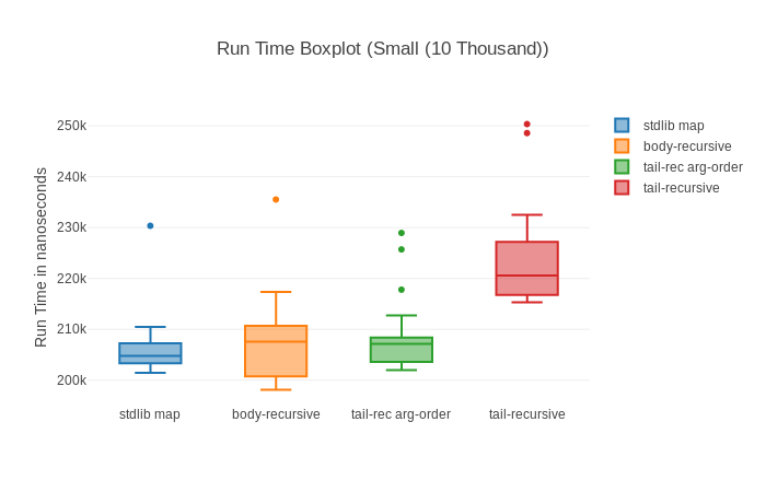
Speaking about spotting, have you noticed anything in those graphs? Almost all of them show that some big outliers might be around screwing with our results. The basic comparison shows pretty big standard deviation, the box plot one straight up shows outliers (little dots), the histogram show that for a long time there’s nothing and then there’s a measurement that’s much higher and in the raw run times we also see one enormous spike.

All of this is even more prevalent when we look at the graphs for the small input (10 000 elements):

Why could this be? Well, my favourite suspect in this case is garbage collection. It can take quite a while and as such is a candidate for huge outliers – the more so the faster the benchmarks are.

So let’s try to take garbage collection out of the equation. This is somewhat controversial and we can’t take it out 100%, but we can significantly limit its impact through benchee’s hooks feature. Basically through adding after_each: fn _ -> :erlang.garbage_collect() end to our configuration we tell benchee to run garbage collection after every measurement to minimize the chance that it will trigger during a measurement and hence affect results.

You can have a look at it in this HTML report. We can immediately see in the results and graphs that standard deviation got a lot smaller and we have way fewer outliers now for our smaller input sizes:

Note however that our sample size also went down significantly (from over 20 000 to… 30) so increasing benchmarking time might be worth while to get more samples again.

How does it look like for our big 5 Million input though?

Not much of an improvement… Actually slightly worse. Strange. We can find the likely answer in the raw run time graphs of all of our contenders:

The first sample is always the slowest (while running with GC it seemed to be the third run). My theory is that for the larger amount of data the BEAM needs to repeatedly grow the memory of the process we are benchmarking. This seems strange though, as that should have already happened during warmup (benchee uses one process for each scenario which includes warmup and run time). It might be something different, but it very likely is a one time cost.

To GC or not to GC

Is a good question. Especially for very micro benchmarks it can help stabilize/sanitize the measured times. Due to the high standard deviation/outliers whoever is fastest can change quite a lot on repeated runs.

However, Garbage Collection happens in a real world scenario and the amount of “garbage” you produce can often be directly linked to your run time – taking the cleaning time out of equation can yield results that are not necessarily applicable to the real world. You could also significantly increase the run time to level the playing field so that by the law of big numbers we come closer to the true average – spikes from garbage collection or not.

Wrapping up

Anyhow, this was just a little detour to show how some of these graphs can help us drill down and find out why our measurements are as they are and find likely causes.

The improvements in benchee mean the promotion of better practices and much less manual work. In essence I could just link the HTML report and then just discuss the topic at hand (well save the benchmarking code, that’s not in there… yet 😉 ) which is great for publishing benchmarks. Speaking about discussions, I omitted the discussions around tail recursive calls etc. with comments from José Valim and Robert Virding. Feel free to still read the old blog post for that – it’s not that old after all.

Happy benchmarking!

Released: benchee 0.99, 1.0 & friends

It’s finally here – benchee 1.0! 🎉🎉🎉

The first benchee release was almost 3 years ago – it started a mission to improve benchmarking tooling in the elixir eco system. And now we’re not at the goal – after all it’s never done and we’re not short of ideas of what to do.

What’s in a 1.0?

Also called “Why did you take so long to call it 1.0?” – 1.0 for me means a good level of stability. A level where not every second new benchee version all formatters would need updates because they would break otherwise. And in recent releases we have still shuffled major data structures around A LOT (just check all the Breaking Changes (Plugins)). Benchee was mostly stable from a user perspective – but this means it’s less of a risk factor to go ahead and write your own plugins, something that benchee always encouraged/was built to empower. I don’t have any plans for 2.0 right now – all features that I know of can easily be added to the existing structure.

It also means I’m happy with the features. What benchee offers is great, we have:

•  nano second precise run time measurements
•  memory measurements
• rich statistics
• show information such as CPU, elixir and erlang versions about the system running the benchmarks
•  support for multiple inputs
•  hooks to support even unconventional scenarios
• you can access it all via your CLI, CSV, JSON or HTML (including nice graphs!)
• and actually a lot more 😉

Benchee might have started out as “I want benchmark-ips in elixir” but it has surpassed it in many ways so that I’d actually want to have benchee in Ruby but that’s another topic. However, that makes me proud of what we accomplished.

With that amount of polish I can also easily sit back and not work on benchee for some time because I know it’s good – it is “done” in the sense that it can do everything I wanted it to do when I started the project (and even more!).

As for what is actually in it mostly removing deprecations. You can check out the Changelog.

What’s 0.99?

I found it nice how rspec did their 2.99 –> 3.0 switch – get it to run on 2.99 without deprecation warnings and then you can safely use 3.0. That was a great user experience. Ember.js handles their major versions similarly. Now, benchee is nowhere near as complex as those 2 but we thought providing that nicety would still be great.

Features

As mentioned before 0.99/1.0 don’t actually include many features – the previous 0.14.0 release from about a month ago was very feature packed. These releases are a lot about polish. Redoing the documenation, updating names, fixing typespecs, being more careful about what is and isn’t exposed in the public interface.

A small but important feature made it in though – displaying the absolute difference between measurements:

Comparison:
flat_map           2.34 K
map.flatten        1.22 K - 1.92x slower +393.09 μs

See that little+393.09 μs? It’s how much slower it was on average in absolute terms. With these comparisons people often focus too much on “OMG it’s almost 2 times as slow!!!” but this number helps put it into context: It’s not even half a millisecond. If you only do this once in a web request the difference likely doesn’t matter. It’s a calculation I always did in my head, I’m happy to make it easily accessible for everyone.

Along with this patch those values were added to our Statistics struct – including the “x-times slower” values, which means formatters no longer have to implement this themselves! Hooray!

We’re an org now!

An astute observer might have seen that all my benchee repos have been moved to the github organization bencheeorg. What’s that all about? It’s mostly a tribute to benchee not being a personal project but a community project. Many people have contributed massively to benchee, most notably Devon and Eric. Without Devon we probably still wouldn’t have memory measurements and without Eric our unit scaling wouldn’t be as great as it is. Others such as Michał and OvermindDL1 have also contributed a lot through ideas, testing and help (especially with memory measurements :)). Feels wrong to keep the repositories attached to a single person.

Also, should anything happen to me (which I hope won’t happen), the others could still add people to the organization and carry on.

It also helps with another problem I’ve had: I want to extract small useful libraries from benchee: Statistics (introduced by me), System Information gathering (introduced by Devon) and unit scaling (introduced by Eric) – where do I put these repos? All under their own name space? All under my name space? Nah, I put them in the benchee organization where we share ownership – that’s where they belong.

The future of benchee

As I said benchee isn’t done – there is an open PR to add reference jobs which didn’t make it into the release. We’d like to add more types of memory measurements, as well as measuring reductions, incorporating profiling right after benchmarking to drill down on those bottle necks sounds great, more compact console output and also include the benchmarking code itself in the suite so that formatters could display it. Finally, now might finally be the time to brush up on meta programming and write that DSL wrapper that people apparently want.

Help with all of those is very welcome. Personally, I’m really itching to extract these libraries I mentioned – let’s see about that. Also to showcase benchee with some nice benchmarks – after all what good is a great benchmarking tool if you rarely use it?

Released: benchee 0.10, HTML, CSV and JSON plugins

It’s been a little time since the last benchee release, have we been lazy? Au contraire mes ami! We’ve been hard at work, greatly improving the internals, adding a full system for hooks (before_scenarion, before_each, after_each, after_scenario) and some other great improvements thanks to many contributions. The releases are benchee 0.10.0 (CHANGELOG), benchee_csv 0.7.0 (CHANGELOG), benchee_html 0.4.0 (CHANGELOG) and benchee_json 0.4.0 (CHANGELOG).

Sooo… what’s up? Why did it take so long?

benchee

Before we take a look at the exciting new features, here’s a small summary of major things that happened in previous releases that I didn’t manage to blog about due to lack of time:

0.7.0 added mainly convenience features, but benchee_html 0.2.0 split up the HTML reports which made it easier to find what you’re looking for but also alleviated problems with rendering huge data sets (the graphing library was reaching its limits with that many graphs and input values)

0.8.0 added type specs for the major public functions, configuration is now a struct so errors out on unrecognized options

0.9.0 is one of my favorite releases as it now gathers and shows system data like number of cores, operating system, memory and cpu speed. I love this, because normally when I benchmark I and write about it I need to write it up in the blog post. Now with benchee I can just copy & paste the output and I get all the information that I need! This version also facilitates calling benchee from Erlang, so benchee:run is in the cards.

Now ahead, to the truly new stuff:

Scenarios

In benchee each processing step used to have its own main key in the main data structure (suite): run_times, statistics, jobs etc. Philosophically, that was great. However, it got more cumbersome in the formatters especially after the introduction of inputs as access now required an additional level of indirection (namely, the input). As a result, to get all the data for a combination of job and input you want to format you have got to merge the data of multiple different sources. Not exactly ideal. To make matters worse, we want to add memory measurements in the future… even more to merge.

Long story short, Devon and I sat down in person for 2 hours to discuss how to best deal with this, how to name it and all accompanying fields. We decided to keep all the data together from now on – for every entry of the result. That means each combination of a job you defined and an input. The data structure now keeps that along with its raw run times, statistics etc. After some research we settled on calling it a scenario.

	defmodule Benchee.Benchmark.Scenario do
	@moduledoc """
	A Scenario in Benchee is a particular case of a whole benchmarking suite. That
	is the combination of a particular function to benchmark (`job_name` and
	`function`) in combination with a specific input (`input_name` and `input`).
	It then gathers all data measured for this particular combination during
	`Benchee.Benchmark.measure/3` (`run_times` and `memory_usages`),
	which are then used later in the process by `Benchee.Statistics` to compute
	the relevant statistics (`run_time_statistics` and `memory_usage_statistics`).
	"""
	@type t :: %__MODULE__{
	job_name: binary,
	function: fun,
	input_name: binary | nil,
	input: any | nil,
	run_times: [float] | [],
	run_time_statistics: Benchee.Statistics.t | nil,
	memory_usages: [non_neg_integer] | [],
	memory_usage_statistics: Benchee.Statistics.t | nil,
	before_each: fun | nil,
	after_each: fun | nil,
	before_scenario: fun | nil,
	after_scenario: fun | nil
	}
	end

view raw

benchee_scenario.ex

hosted with ❤ by GitHub

This was a huge refactoring but we really like the improvements it yielded. Devon wrote about the refactoring process in more detail.

It took a long time, but it didn’t add any new features – so no reason for a release yet. Plus, of course all formatters also needed to get updated.

Hooks

Another huge chunk of work went into a hooks system that is pretty fully featured. It allows you to execute code before and after invoking the benchmark as well as setup code before a scenario starts running and teardown code for after a scenario stopped running.

That seems weird, as most of the time you won’t need hooks. We could have released with part of the system ready, but I didn’t want to (potentially) break API again and so soon if we added arguments or found that it wasn’t quite working to our liking. So, we took some time to get everything in.

So what did we want to enable you to do?

• Load a record from the database in before_each and pass it to the benchmarking function, to perform an operation with it without counting the time for loading the record towards the benchmarking results
• Start up a process/service in before_scenario that you need for your scenario to run, and then…
• …shut it down again in after_scenario, or bust a cache
• Or if you want your benchmarks to run without a cache all the time, you can also bust it in before_each or after_each
• after_each is also passed the return value of the benchmarking function so you can run assertions on it – for instance for all the jobs to see if they are truly doing the same thing
• before_each could also be used to randomize the input a bit to benchmark a more diverse set of inputs without the randomizing counting towards the measured times

All of these hooks can be configured either globally so that they run for all the benchmarking jobs or they can be configured on a per job basis. The documentation for hooks over at the repo is a little blog post by itself and I won’t repeat it here 😉

As a little example, here is me benchmarking hound:

	# ATTENTION: gotta start phantomjs via `phantomjs –wd` first..
	Application.ensure_all_started(:hound)
	{:ok, server} = SimpleServer.start
	Application.put_env(:hound, :app_host, "http://localhost")
	Application.put_env(:hound, :app_port, SimpleServer.port(server))
	use Hound.Helpers
	Benchee.run(%{
	"fill_in text_field" => fn ->
	fill_field({:name, "user[name]"}, "Chris")
	end,
	"visit forms" => fn ->
	navigate_to("#{server.base_url}/forms.html")
	end,
	"find by css #id" => fn ->
	find_element(:id, "button-no-type-id")
	end
	},
	time: 18,
	formatters: [
	Benchee.Formatters.HTML,
	Benchee.Formatters.Console
	],
	html: [file: "benchmarks/html/hound.html"],
	before_scenario: fn(input) ->
	Hound.start_session()
	navigate_to("#{server.base_url}/forms.html")
	input
	end,
	after_scenario: fn(_return) ->
	Hound.end_session
	end)

view raw

benchee_hound.exs

hosted with ❤ by GitHub

Hound needs to start before we can benchmark it. Howeer, hound seems to remember the started process by the pid of self() at that time. That’s a problem because each benchee scenario runs in its own process, so you couldn’t just start it before invoking Benchee.run. I found no way to make the benchmark work with good old benchee 0.9.0, which is also what finally brought me to implement this feature. Now in benchee 0.10.0 with before_scenario and after_scenario it is perfectly feasible!

Why no 1.0?

With all the major improvements one could easily call this a 1.0. Or 0.6.0 could have been a 1.0 then we’d be at 2.0 now – wow that sounds mature!

Well, I see 1.0 as a promise – a promise for plugin developers and others that compatibility won’t be broken easily and not soon. Can’t promise this when we just broke plugin compatibility in a major way. That said, I really feel good about the new structure, partly because we put so much time and thought into figuring it out, but also because it has greatly simplified some implementations and thinking about some future features it also makes them a lot easier to implement.

Of course, we didn’t break compatibility for users. That has been stable since 0.6.0 and to a (quite big) extent beyond that.

So, 1.0 will of course be coming some time. We might get some more bigger features in that could break compatibility (although I don’t think they will, it will just be new fields):

• Measuring memory consumption
• recording and loading benchmarking results
• … ?

Also before a 1.0 release I probably want to extract more not directly benchmarking related functionality from benchee and provide as general purpose libraries. We have some sub systems that we build for us and would provide value to other applications:

• Unit: convert units (durations, counts, memory etc.), scale them to a “best fit” unit, format them accordingly, find a best fit unit for a collection of values
• Statistics: All the statistics we provide including not so easy/standard ones like nth percentile and mode
• System: gather system data like elixir/erlang version, CPU, Operating System, memory, number of cores

Thanks to the design of benchee these are all already fairly separate so extracting them is more a matter of when, not how. Meaning, that we have all the functionality in those libraries that we need so that we don’t have to make a coordinated release for new features across n libraries.

benchee_html

Especially due to many great community contributions (maybe because of Hacktoberfest?) there’s a number of stellar improvements!

• System information is now also available and you can toggle it with the link in the top right
• unit scaling from benchee “core” is now also used so it’s not all in micro seconds as before but rather an appropriate unit
• reports are automatically opened in your browser after the formatter is done (can of course be deactivated)
• there is a default file name now so you don’t HAVE to supply it

What’s next?

Well this release took long – hope the next one won’t take as long. There’s a couple of improvements that didn’t quite make it into the release so there might be a smaller new release relatively soon. Other than that, work on either serializing or the often requested “measure memory consumption” will probably start some time. But first, we rest a bit 😉

Hope you enjoy benchmarking and if you are missing a feature or getting hit by a bug, please open an issue ❤